OpenGL Project

Introduction

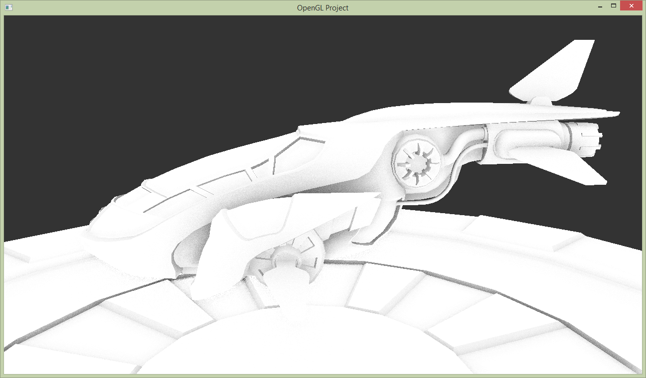
In tutorial 4, we calculate the indirect illumination (from the environment) with two terms. One of the terms, the diffuse illumination, is the irradiance (energy per area) that comes from the whole hemisphere around the surface normal. We then assume that all light from the hemisphere actually reaches the fragment, but there may be geometry that occludes (blocks) the sky (see the image below). In this project, we will compute the hemispherical occlusion by looking at nearby depth values in the z-buffer, a method called Screen Space Ambient Occlusion (SSAO). The result is visualized in the image above.

In other words, for each pixel we want to estimate how much of the hemisphere is occluded, and then we attenuate the diffuse indirect illumination by that. Traditional Ambient Occlusion (AO), where you shoot a bunch of rays to estimate the occlusion, has been a popular way of "faking" full global illumination calculations for a very long time, and was even used in the movie industry until quite recently. In video games, shooting a large number of rays per pixel is infeasible, but in 2007 the SSAO technique was developed and first used in a game ("Crysis").

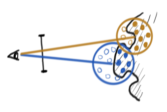
The idea was to precompute a number (e.g., 16) of uniformly distributed samples, $s_i$ in a sphere. Then, for each pixel at position $p$ we want to know how many of those samples are blocked from the light (if 50% are blocked, we will attenuate indirect illumination by 50%). To be able to do this the people at Crytek tried a horrendous hack: They simply calculate $p + s_i$ and project that point onto the image plane. If the projected point has a depth that is further away than the corresponding value in the depth buffer, the point is considered blocked (see the top image to the right). This turned out to be extremely cheap and look surprisingly good, and today there are hardly any games that ship without some sort of SSAO technique.

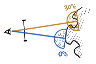
There are a million different extensions and variations of this algorithm, and if you find a version you would rather try, ask an assistant if that's allright. Otherwise, we're going to do it the Crysis way, with two important improvements. First, with the original algorithm, if $p$ lies on a plane, 50% of the samples will always be covered. Therefore we will instead generate samples in a hemisphere and transform them using the pixel's normal (see the second image to the right).

Since we precompute a number of well-distributed samples and then use the same samples for every pixel, there will be a lot of aliasing in the final result. To get rid of this, a common trick is to rotate the samples around the normal with a random rotation for each pixel.

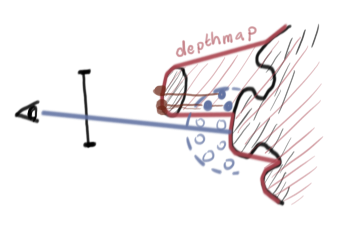
Secondly, the depth map does not really contain enough information for what we want to test. Consider the third image to the right. Three of the samples will be considered "blocked" because they lie behind the depth map, but the corresponding samples in the depth map are actually far away, and might not block $p$ at all. Therefore, once we have the depth of a "blocking" sample, we decide whether the sample lies within the hemisphere and if it doesn't we ignore that sample.

Guidelines

You may now go ahead and implement this however you choose to, but in this section we will suggest an overview of the steps you could take to get it working, along with some generally useful code snippets.

Generate a bunch of uniformly distributed samples, $s_i$, in the unit hemisphere. This is done once on the CPU, before you start any rendering, and then the samples are sent into the shader as a uniform array of vec3. There is a function labhelper::coseineSampleHemisphere() which you can use to get nicely distributed samples on the hemisphere, and then you can use labhelper::randf() to randomly scale their length.
Generate a texture with random angles to rotate the samples by. This can be a fairly small texture (e.g., 64x64) and then you use GL_REPEAT to make sure every pixel gets a value.
Render the depth and normal to a framebuffer. Just render the scene once to a separate framebuffer using a different shader program which simply writes the view-space normal as the color. The depth will be stored in the attached depth-buffer.
Compute the SSAO in a post-processing pass. This is the tricky part. You will render a fullscreen pass, and for every fragment you can fetch the depth and normal from the previous pass. The SSAO result is stored in a new texture. Some tips and details are given below.
Render the scene with shading as usual, but scale the diffuse indirect term with the SSAO term. The output from the previous SSAO pass is passed in as a texture to your standard shader, and you simply read the SSAO value from that, for each fragment.

We suggest that you start by ignoring the rotation part until everything else works. Also, visualize the result from the SSAO pass until it works and then use it to attenuate the shading. It might also be helpful to add some global variables (e.g., number of samples, sample radius and whether to use SSAO at all) and create GUI sliders for them.

Details

We will compute the hemispherical occlusion in a postprocess pass, saving the output to a dedicated framebuffer. For each pixel in the SSAO pass, we first determine the view-space position and view-space normal. The normal can be directly fetched from the pre-pass framebuffer texture, and the position can be computed from the depth buffer:

float fragmentDepth = texture(depthTexture, texCoord).r;

// Normalized Device Coordinates (clip space)
vec4 ndc = vec4(texCoord.x * 2.0 - 1.0, texCoord.y * 2.0 - 1.0, 
                fragmentDepth * 2.0 - 1.0, 1.0);

// Transform to view space
vec3 vs_pos = homogenize(inverseProjectionMatrix * ndc);

With the helper function:

vec3 homogenize(vec4 v) { return vec3((1.0 / v.w) * v); }

From this position, we want to sample the depth buffer in a surrounding to see if there are occlusions on the hemisphere. We start by establishing base vectors for the hemisphere in view space. The normal can be used for one of the base vectors, and the other two lie in the tangent plane (orthogonal to the normal) and we can compute the a tangent and bi-tangent:

vec3 vs_tangent = perpendicular(vs_normal);
vec3 vs_bitangent = cross(vs_normal, vs_tangent);

With the helper function:

// Computes one vector in the plane perpendicular to v
vec3 perpendicular(vec3 v)
{
	vec3 av = abs(v); 
	if (av.x < av.y)
		if (av.x < av.z) return vec3(0.0f, -v.z, v.y);
		else return vec3(-v.y, v.x, 0.0f);
	else
		if (av.y < av.z) return vec3(-v.z, 0.0f, v.x);
		else return vec3(-v.y, v.x, 0.0f);
}

And the local base can consist of the tangent, bitangent and the normal:

mat3 tbn = mat3(vs_tangent, vs_bitangent, vs_normal); // local base

Now, we will test $N$ sample offsets in the depth buffer in a for loop:

int num_visible_samples = 0; 
int num_valid_samples = 0; 
for (int i = 0; i < nof_samples; i++) {
	// Project hemishere sample onto the local base
	vec3 s = tbn * samples[i];

	// compute view-space position of sample
	vec3 vs_sample_position = vs_pos + s * kernel_size;

	// compute the ndc-coords of the sample
	vec3 sample_coords_ndc = homogenize(projectionMatrix * vec4(vs_sample_position, 1.0));

	// Sample the depth-buffer at a texture coord based on the ndc-coord of the sample
	float blocker_depth = texture(...)

	// Find the view-space coord of the blocker
	vec3 vs_blocker_pos = homogenize(inverseProjectionMatrix * 
	     vec4(sample_coords.xy, blockerDepth * 2.0 - 1.0, 1.0));	

	// Check that the blocker is closer than kernel_size to vs_pos
	// (otherwise skip this sample)

	// Check if the blocker pos is closer to the camera than our
	// fragment, otherwise, increase num_visible_samples

	num_valid_samples += 1;
}

float hemisphericalVisibility = float(num_visible_samples) / float(num_valid_samples);

if (num_valid_samples == 0)
	hemisphericalVisibility = 1.0;

Tip: After projecting and homogenizing a view-sample point, you will have coordinates in the $(-1,-1,-1)-(1,1,1)$ range. To sample a texture you need to convert these to the $(0,0,0)-(1,1,1)$ range.

Once this works and looks believable, add the per-pixel random rotation. You pick a random value per pixel from a texture, and then rotate your tbn base around the normal (so you will need to create a rotation matrix that rotates around the z-axis).

Optional

When you are done, you should have an SSAO solution that gives nice looking results if you take many samples per pixel. In reality, you can really only afford a few, so common practice is to generate noisy results with a few samples and then doing a bilateral blur in the SSAO output before using it. Give that a try if you have time.