Introduction

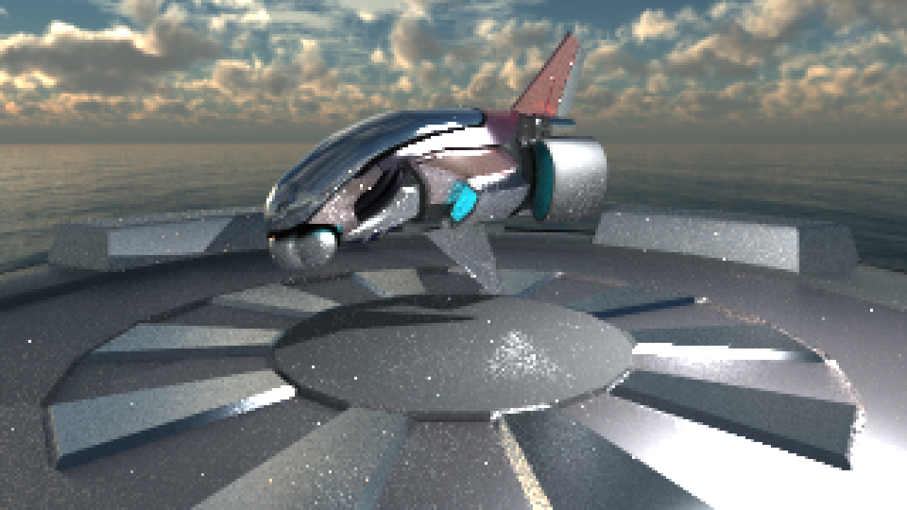
In this final project you will write a path tracer capable of rendering photorealistic images (if fed with something more photorealistic than a weird spaceship). The focus here will be on correctness, rather than speed and, unlike the images you have rendered in previous labs, which are complete in a few milliseconds, you may have to wait for hours for your best work to look really good. Path tracing is one of many algorithms used for offline rendering, e.g., when rendering movies.

Path tracing is based on the concept of "ray tracing", rather than "rasterization", which is what you have done so far and what GPUs do so well. Ray tracing is when we intersect a ray with a virtual scene and use the intersection points to calculate the light coming from that direction. In this tutorial, the actual ray tracing will be done using Intel's "Embree" library, and we will focus on how to generate physically plausible images.

There will be a relatively large amount of theory in this tutorial, and some scary looking maths, but please DON'T PANIC. The idea is that you shall get a feel for how the underlying maths work, but you will not be asked to solve anything especially difficult.

The startup code

The first thing you should do (after having pulled the latest code) is to set the Pathtracer as startup project and switch to Release. Since the algorithm is highly CPU bound, this code will run extremely slow in Debug, both because no optimizations are turned on, and because we run on a single thread in the Debug build. So, always run it in Release, except when you have to actually run the debugger.

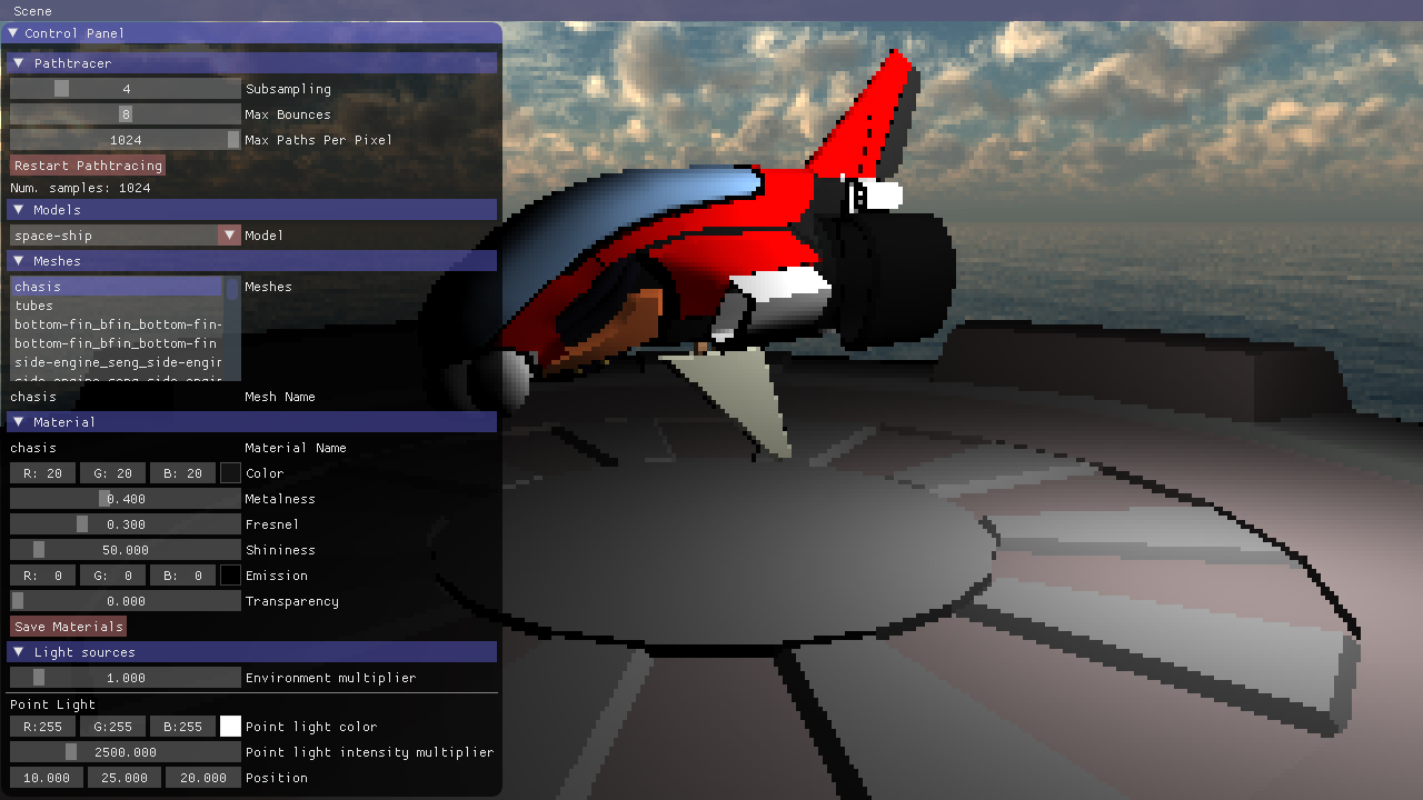
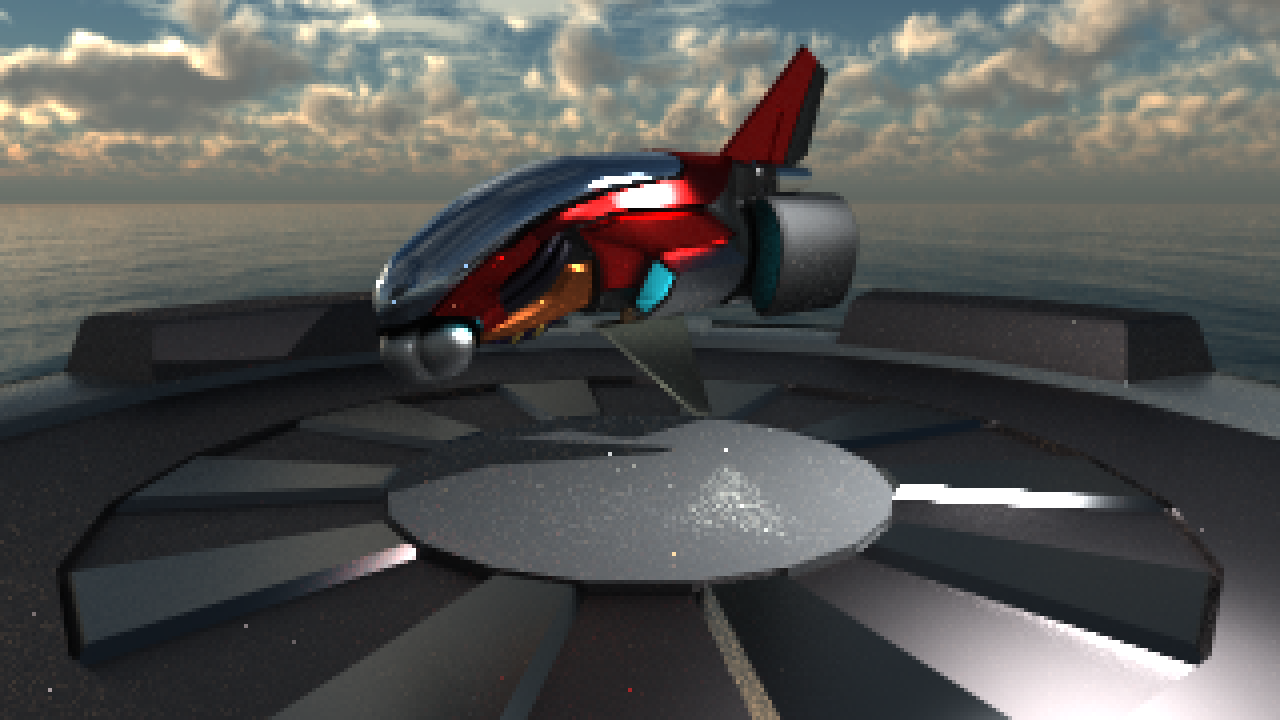
Now run the program. Except for it being slower and lower resolution, you will see what should be a familiar scene by now.

You will recognize the GUI from Tutorial 4, but there are a few changes. You can now load several .obj models, and you can choose which you want to edit the materials for in the first drop-down list. There are also a few new settings for the path tracer. Right now, the most important one is the subsampling setting. It determines how many window pixels (w x h) a pixel in the raytraced image should correspond to. You may want to increase this value if you find the program to be irresponsive. The Max Bounces slider doesn't do anything yet, but you will use it later. The Max Paths Per Pixel looks like it doesn't do anything yet, but it actually says how many frames the renderer should calculate and accumulate. It will be useful later, e.g., to be able to compare images with the same quality. When it is set to zero, it will accumulate the result until you close the program (or the rendering is restarted by pressing the button or changing the viewpoint).

The difference is that this image is ray traced. The only thing we use OpenGL for in this program is to render a fullscreen quad, textured with the output from your raytracer (and to render the GUI, obviously). The actual image is created on the CPU by shooting one ray for every pixel and intersecting it with the scene to find the closest intersection. For that intersection, a color is calculated and accumulated to the pixel in the rendered image.

Now let's take a look at the code, and make sure you understand how the image is generated.

• main.cpp: This should be familiar. A simple OpenGL program that draws a full-screen quad each frame and renders a GUI.
• pathtracer.h/cpp: This is where the interesting stuff happens. Look at tracePaths(): this code loops through all the pixels and shoots a ray for each to find an intersection point. Then the Li() function is called to calculate the incoming radiance for the intersected point. This function is where you will focus most of your efforts.
• embree.h/cpp: The raytracing is handled by the external library "Embree". These files serve as an interface to that library. Have a look at the .h file and make sure you understand what each function does. How it does it is less important for this tutorial.
• material.h/cpp: These files define the BRDFs that we will use. We will explain further how everything in here works in a while.
• sampling.h/cpp: Some helper functions for sampling random distributions.

Tasks

Improve the ray tracer

Before we go into path tracing, let's improve this raytracer a bit.

Jittered Sampling

We will begin with some much needed anti-aliasing. Look at the tracePaths() function again. Every frame, we create a ray that goes through each pixel, and then we accumulate the result to the result of previous frames. Start by changing the code so that it picks a random direction within each pixel at each frame.

Note that the way we take the samples is by converting the pixel's x,y position from an integer to the corresponding screen space values (in the range -1 to 1), and then applying the inverse projection and view matrices to that, obtaining a world-space position. Right now, we always take the same position for each pixel, corresponding to the integral part of the pixel. You need to change this so we take different positions inside each pixel instead.

Shadows

Take a closer look at the Li() function. To calculate the color of each pixel, this code does pretty much what you started with in Tutorial 4. That is, it calculates the incoming radiance from the light and multiplies this by the cosine term and the diffuse BRDF. To add shadows, you need to shoot a ray starting at the intersected point and going towards the light source, and find out if there is something occluding the point. Use the occluded() function, rather than intersect(). Why do you think we need both of these functions?

The material model

We use a material model loosely based on that of pbrt. Specifically, we define 3 interfaces: BSDF, BRDF, and BTDF, corresponding to the Bidirectional Distribution Functions for Scattering, Reflection and Transmission, respectively.

Initially we will only define a single BTDF, that for the diffuse, which simulates subsurface scattering of the light by reflecting it in a uniformly random direction. In the last part of this project, where you implement something by yourself, you may choose to implement a refractive material, which you can implement as another child of this interface.

The BRDF interface is used for the actual reflections on the surface. We will use a microfacet model here, but other reflection models could be implemented instead, such as using perfect reflections.

Finally, the BSDF interface represents the entire surface interaction. In our case, we will have two of these, one for dielectric materials, which will mix results between a BTDF and a BRDF, and one for metallic materials, which only uses a BRDF as, in general, light doesn't get transmitted through metals, only absorbed or reflected.

All these classes have 2 main functions:

• f, which will return a color by which the light is modified, given an incoming and outgoing directions, and the normal of the surface.
• sample_wi, which we will use later to calculate new directions to follow after the light interacts with the surface.

Blinn-Phong Microfacet BRDF

Yes, "again"! But this time you need to squeeze it into our nice little material tree. Take a look at the Li() function again. One of the first things we do is to define an object mat of the type BTDF. This is the object that we will use throughout the function to evaluate the BSDF and to sample directions. Currently it is a simple object of type Diffuse (which inherits BTDF). Change it to use the dielectric BSDF instead, with a microfacet BRDF, which will reflect diffusely the energy that is refracted by the surface.

Diffuse diffuse(hit.material->m_color);
MicrofacetBRDF microfacet(hit.material->m_shininess);
DielectricBSDF dielectric(&microfacet, &diffuse, hit.material->m_fresnel);
BSDF& mat = dielectric;

If you run the code now, everything will be black, since neither the MicrofacetBRDF nor the DielectricBSDF classes are implemented yet.

Before you start doing that though, go to main.cpp, at the end of the initialize() function, and switch to only loading the simple Sphere model:

//changeScene("Ship");
changeScene("Sphere");

We know that when light interacts with a surface, it is either reflected or refracted depending on the Fresnel equations. We have separated the Fresnel term calculation to its own function, BSDF::fresnel(), because we will need it in several places. Start by implementing that so that it follows the fresnel equation:

where \(\omega_h\) is the half-vector between \(\omega_i\) and \(\omega_o\).

Now let's continue with the DielectricBSDF::f() method. This will mix the values of the reflected and refracted lights using the fresnel term. Specifically:

With this, you should be able to get back some color to the scene, but let's get on the reflections now. Let's now implement the MicrofacetBRDF::f() function. As in lab 4, the immediately reflected light should be:

where \(s\) is the material shininess. Note that in lab 4 we also had the \(F(\omega_i)\) term multiplying here, but we take care of that in the BSDF instead.

When you're done, if the sphere material is set up as below, you should have something like the following result:

The material stack

Now let's put the rest of the material model in place. In Li(), build a complete material like this:

Diffuse diffuse(hit.material->m_color);
MicrofacetBRDF microfacet(hit.material->m_shininess);
DielectricBSDF dielectric(&microfacet, &diffuse, hit.material->m_fresnel);
MetalBSDF metal(&microfacet, hit.material->m_color, hit.material->m_fresnel);
BSDFLinearBlend metal_blend(hit.material->m_metalness, &metal, &dielectric);
BSDF& mat = metal_blend;

Make sure you understand what you copied

Now we need to implement the metal BSDF as well as the linear blend function. Let's start with the LinearBlend::f(): class holds two objects of type BSDF, the idea is that it does a linear blend between the result of those with a weight of w, so you need to call f() in both and return the weighted average.

Finally, let's get the MetalBSDF::f() implemented. This should be similar to what you did for the DielectricBSDF::f(), but remember that the energy that is refracted into a metal is just absorbed and turned into heat, so you only need to obtain the result of the reflection part of the interaction, but a metal tint the light that's reflected from it, so multiply it by the color.

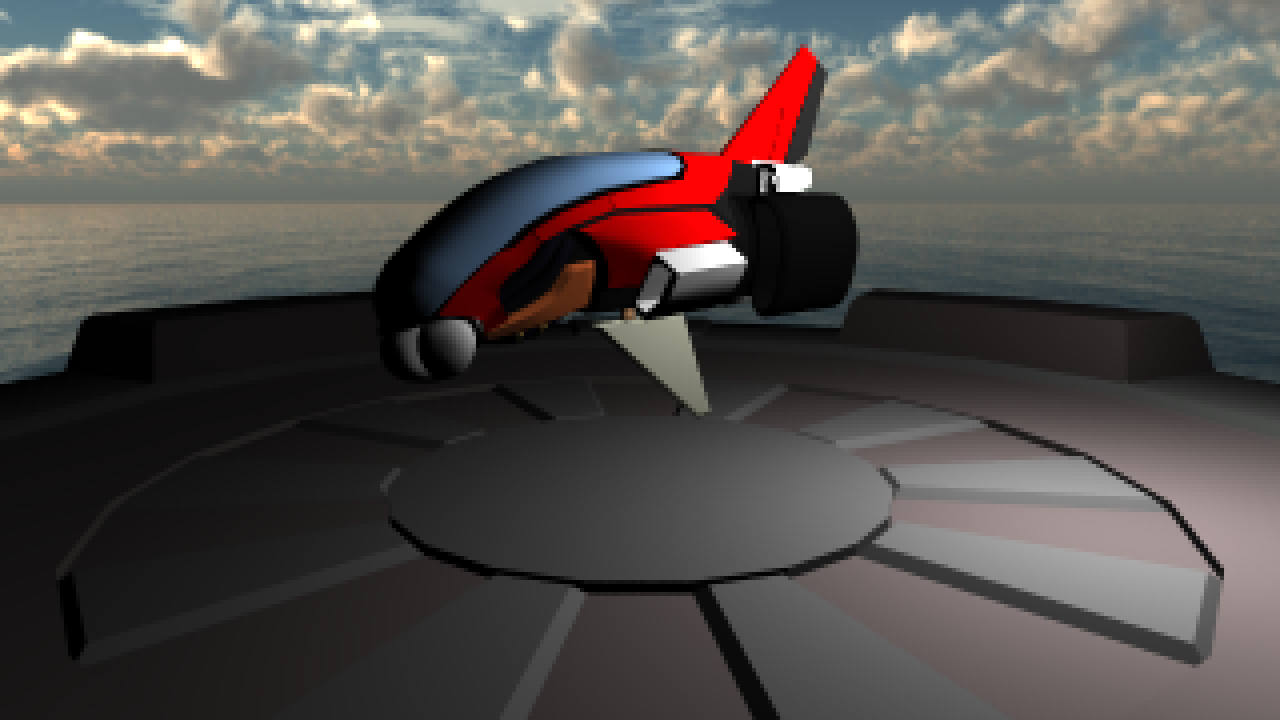
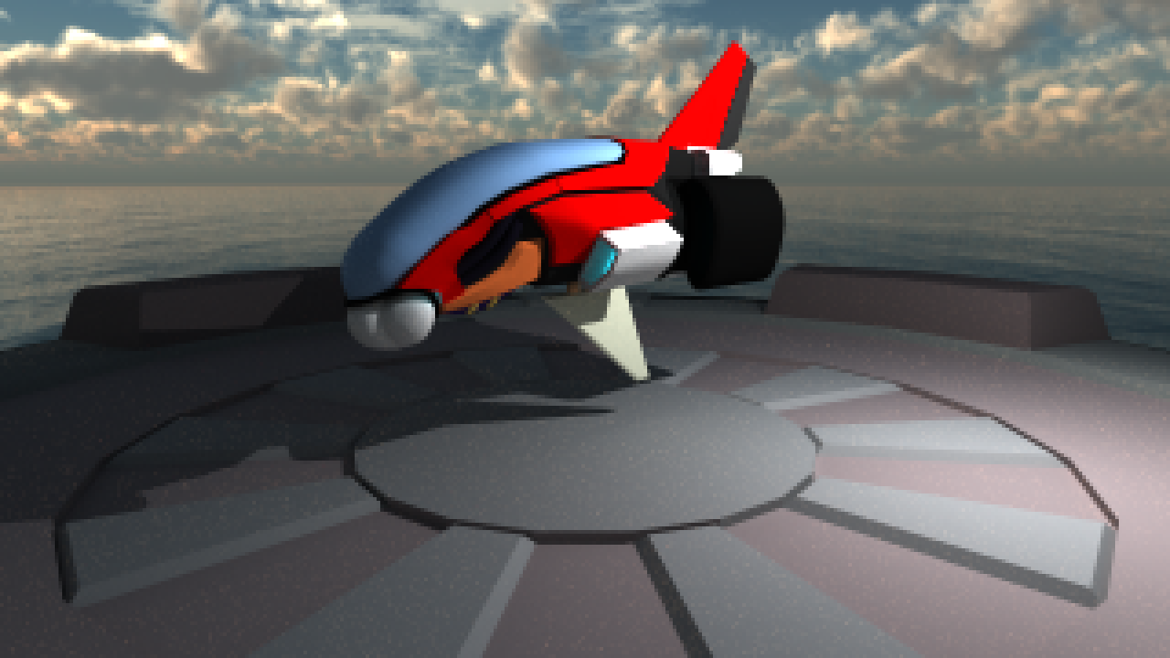
When done, load the Ship scene again and be slightly dissapointed that everything looks a bit boring when you only do direct illumination.

Write a path tracer

Now we are going to turn this simple ray tracer into a full path tracer and get some proper indirect illumination into our immages. At this point there is no way to proceed without first understanding the basics of:

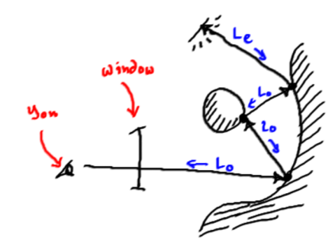
The Rendering Equation

This is a formula that tells us what the outgoing radiance from some point will be, given that we know all the incoming radiance at that point. If you need more details than given here, have a look at lectures 8 and 9, and their related material in the textbook, or cruise the internet. The equation looks like this (we have omitted the point, \(p\), for brevity):

It says that the radiance (Watt per unit solid angle and unit area) \(L_o\) that leaves a point in the direction \(\omega_o\) can be found from the:

• Emitted Light: \(L_e(\omega_o)\) - If the surface at this point emits radiance in direction \(\omega_o\).
• BRDF: \(f(\omega_i, \omega_o)\) - This is a function that describes how the surface at this point reflects light that comes from direction \(\omega_i\) in direction \(\omega_o\).
• Incoming radiance: \(L_i(\omega_i)\) - This is the incoming light from direction \(\omega_i\).
• Cosine term: \(cos(n, \omega_i)\) - This will attenuate the incoming light based on the incident angle.

There is no analytical solution to this equation. We can however estimate it using what is called Monte Carlo integration, and that is exactly what a path tracer does.

Without going into too much detail, monte carlo integration means that we can get what is called an unbiased estimator of the integral by sampling one direction \(\omega_i\) randomly, if we then weight our estimate by the Probability Density Function, or PDF. The PDF is (roughly) a function that tells us how likely we were to choose the random direction \(\omega_i\).

The fact that it is an unbiased estimator means that if we calculate:

we can get the correct outgoing radiance as:

if we take an infinite number of samples. And a very good estimation if we take "enough" samples.

At some intersection point, we can immediately evaluate everything in Equation 1, above, except for the \(L_i(\omega_i)\) term (the incoming light from direction \(\omega_i\)). But the incoming radiance from some direction can be found by shooting a ray in that direction, and calculating the outgoing radiance from the closest intersecting point. And we know how to estimate the outgoing radiance at that point by looking in a single new incoming direction.

Path tracing

What all this boils down to is the path tracing algorithm. We start by shooting one ray per pixel (the ray starts at the camera position and goes "through" the pixel and into the scene). We find the closest intersection point with the scene and we want to estimate the outgoing radiance from there towards the pixel.

We can do so by shooting one single ray to estimate the incoming radiance.

At the closest intersection point for that new ray, we again shoot a single ray, and keep repeating the process, thus forming a path that goes on until there is no intersection (or we terminate on some other criteria).

At each vertex of the path we will evaluate the emitted light, the BRDF and the cosine term to obtain the radiance reflected at the point.

When the recursion has terminated and we have obtained \(L_o\) for the first ray shot, we record this radiance in the pixel.

This is all we need to do to create a mathematically sound estimation of the true global illumination image we sought! It's probably all black though, unless we were lucky and hit an emitting surface with some rays, in which case it might be black with a little bit of noise. But if we keep running the algorithm, and accumulate the incoming radiance in each pixel (and divide by the number of samples) we would eventually end up with a correct image.

This would take more time than is left for this course though, so we need to speed things up a bit.

Separating Direct and Indirect Illumination

The first step is to separate indirect and direct illumination.

At each vertex of the path, we will first shoot a shadow-ray to each of the light-sources in the scene. If there is no geometry blocking the light, we will multiply the radiance from the light with the BRDF and cosine term.

Then, we will add the incoming indirect light by shooting a single ray in a random direction as before. For this to be correct, we just have to make sure that the surfaces we have chosen to be light sources do not contribute emitted radiance if sampled by an indirect ray.

There! That's a path tracer and it generates correct images in a reasonable time.

Implement a path tracer

So, let's turn all that theory into code now. It is tempting to start writing this as a recursive function, but that will not be very efficient, and we will instead suggest an iterative approach as outlined in the pseudo code below:

L               <- (0.0, 0.0, 0.0)
pathThroughput  <- (1.0, 1.0, 1.0)
currentRay      <- primary ray
for bounces = 0 to settings.max_bounces
{
    // Get the intersection information from the ray
    Intersection hit = getIntersection(current_ray);

    // Create a Material tree
    Diffuse diffuse(hit.material->m_color);
    BRDF & mat = diffuse;

    // Direct illumination
    L += pathThroughput * direct illumination from light if visible

    // Add emitted radiance from intersection
    L += pathThroughput * emitted light

    // Sample an incoming direction (and the brdf and pdf for that direction)
    (wi, f, pdf)  <- mat.sample_wi(hit.wo, hit.shading_normal)

    // If the pdf is too close to zero, it means that the current path is extremely
    // unlikely to exist, so we break to avoid numerical instability
    if(pdf < EPSILON) return L;
    
    cosineterm = abs(dot(wi, hit.shading_normal))

    pathThroughput = pathThroughput * (f * cosineterm)/pdf

    // If pathThroughput is zero there is no need to continue, as no more light comes from this path
    if (pathThroughput == (0,0,0)) return L

    // Create next ray on path (existing instance can't be reused)
    currentRay <- Create new ray instance from intersection point in outgoing direction

    // Bias the ray slightly to avoid self-intersection 
    currentRay.o += PT_EPSILON * hit.normal

    // Intersect the new ray and if there is no intersection just
    // add environment contribution and finish
    if(!intersect(currentRay))
        return L + pathThroughput * Lenvironment(currentRay)

    // Otherwise, reiterate for the new intersection
}

Implement this in your Li() function. To keep things simple for now, switch back to the diffuse BTDF material, and you may use the sphere model at first.

Diffuse diffuse(hit.material->m_color);
BTDF& mat = diffuse;

When you are done, you should have a path-traced image looking like this (after it has rendered for a couple of seconds):

And you can start feeling a little bit proud of yourself.

More complex materials

Let's immediately destroy that new-found self-confidence. Change your material model back to the dielectric BSDF material again:

Diffuse diffuse(hit.material->m_color);
MicrofacetBRDF microfacet(hit.material->m_shininess);
DielectricBSDF dielectric(&microfacet, &diffuse, hit.material->m_fresnel);
BSDF& mat = dielectric;

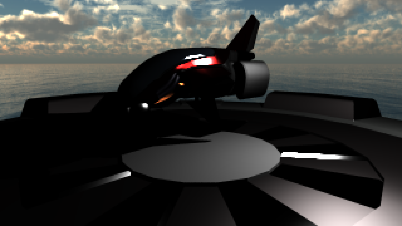
and run the program:

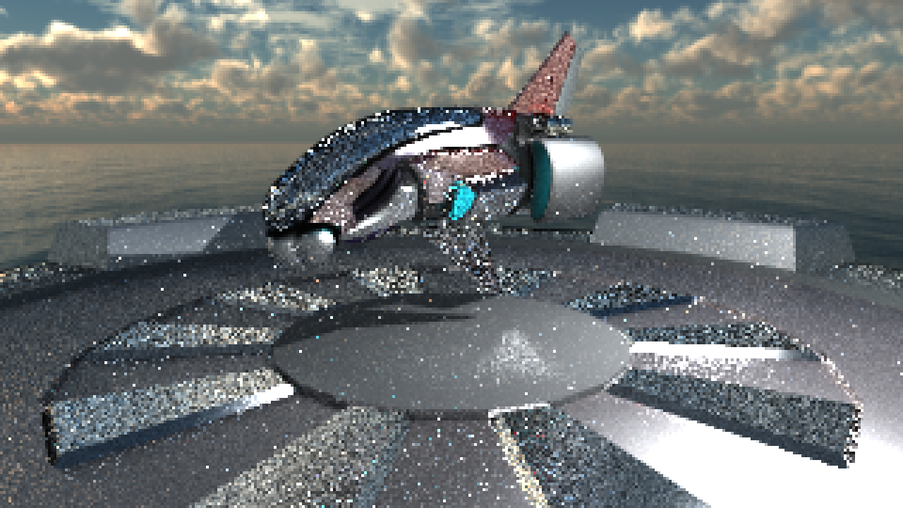
Ouch! That's not what you wanted is it? In theory, there is actually nothing wrong. If you let this image keep rendering you should eventually end up with a nice smooth image, but it could take weeks. This is because of how you choose your incoming direction \(\omega_i\), and the solution is a method called importance sampling.

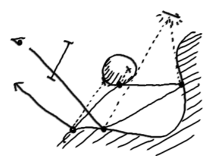
Importance Sampling

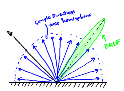
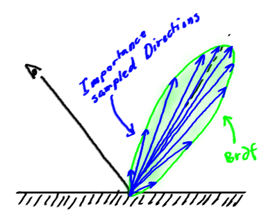
The problem is illustrated in the image to the right. Say that our BRDF represents a near mirror direction. That would mean that all sample directions that are not close to the perfect specular reflection direction will contribute almost nothing. But we still happily choose directions uniformly from all over the hemisphere.

With importance sampling, we will instead pick samples from a distribution that looks more like the BRDF we are trying to integrate, and for which we know the Probability Density Function (PDF), \(p(\omega_i)\).

We will now pick samples with a probability that is much higher for the directions where the BRDF is large. To account for this, we now have to divide the resulting radiance of each sample by the PDF for the sample direction. This means that we will have more samples where the BRDF is high, but if we happen to pick a sample where the PDF is low, its contribution will be increased.

Note that we rarely can find a sampling scheme that exactly matches the BRDF, and that the sampling scheme must be carefully chosen so that it will not occasionally sample directions with very low probability where the BRDF is not correspondingly low. If we did, then we would get very strong samples in some random pixels that take a very long time to converge.

Importance sampling in the BSDF and the Blinn-Phong Microfacet BRDF

Take a look at the current implementation of sample_wi in the DielectricBSDF class. It currently uses sampleHemisphereUniform, which chooses a direction by picking a point uniformly on a disc, and then projecting that onto the hemisphere. This gives the pdf:

This is great for sampling diffuse surfaces, but obviously quite poor for a mirror-like reflection.

So, in what way should we sample the incoming direction? In the best of worlds, we would have a way of choosing directions that had a PDF that was exactly proportional to our complete BSDF. But our BSDF is made up of a combination of BRDF and BTDF, and we don't know what each actually looks like.

Obviously we can't just sample from both and average the result, like we did in the f function, since the average of two vectors taken from different distributions won't represent a correct direction to follow based on any of the two (for an intuitive explanation, think of what would happen if the BRDF was a perfect reflection and the BTDF just let the light pass through the material without modifying it; the average would be a vector that followed the surface of the material, instead of going one of the 2 possible ways).

Instead, we will take a stochastic approach: each time we will decide randomly, with 50% probability, wheter we follow the path of light that is reflected on the surface, or the path that the light takes if the light is refracted. We then include this probability in the PDF by multiplying it by 0.5, and over time, the results will tend to the average we want.

Think about this for a few seconds. We want the function to return a brdf that is: \(F a + (1-F)b\). Instead, after dividing by the pdf, we are going to compute either \(2Fa\) or \(2(1-F)b\). Now, convince yourself that if you do this infinitely many times, the sum of all of those samples is going to be correct. Then start writing your DielectricBSDF::sample_wi function (pseudo code):

if (randf() < 0.5)
{
    // Sample the BRDF
    (wi, pdf, f) <- <...>
    pdf *= 0.5;
    float F = fresnel(wi, wo);
    f *= F;
}
else
{
    // Sample the BTDF
    (wi, pdf, f) <- <...>
    pdf *= 0.5;
    float F = fresnel(wi, wo);
    f *= (1 - F);
}
return (wi, pdf, f)

Great! Now we are sampling from both functions, but if you look at the MicrofacetBRDF::sample_wi you will see that it itself is also sampling the hemisphere uniformly, so we now need to change that in such a way that we get more samples where the BRDF is high.

The actual maths for how to do this is way out of scope for this tutorial, so we will just gloss over it. It is not horribly complicated though, and we will go through it in the "advanced" course. First, we generate a half-angle vector, \(\omega_h\) like this:

WiSample r;
vec3 tangent = normalize(perpendicular(n));
vec3 bitangent = normalize(cross(tangent, n));
float phi = 2.0f * M_PI * randf();
float cos_theta = pow(randf(), 1.0f / (shininess + 1));
float sin_theta = sqrt(max(0.0f, 1.0f - cos_theta * cos_theta));
vec3 wh = normalize(sin_theta * cos(phi) * tangent + 
                    sin_theta * sin(phi) * bitangent + 
                    cos_theta * n);

This vector will be chosen with a pdf:

(Note that the exponent is an \(s\) for "shininess", not an \(8\)).

But what you want is the incoming direction, \(\omega_i\), which you get by reflecting \(\omega_o\) around \(\omega_h\). For reasons that are even more out of scope, the pdf for this vector will be:

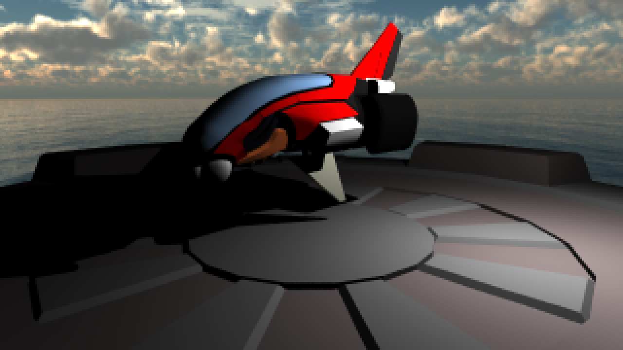
Now plug in your calculations for wi and p in your sample_wi() function and run the program again. After 1024 samples per pixel, it should look something like this:

That's much better, isn't it? There is still noise, of course, but it mostly disappears after a few minutes (or hours, depending on how fast your machine is and how many nasty little bugs are still lying around).

Importance sampling in the LinearBlend and the Metal BSDF

Now we want to turn on the whole material model again. To do that, we need to sample correctly for the BSDFLinearBlend, as well as for the MetalBSDF. Both are fairly simple.

The MetalBSDF is currently sampling with a uniform distribution, as was the case for the dielectric. In this case though, we only have a BRDF to take into account, so the function becomes much simpler. Sample from the underlying BRDF object, and multiply the resulting f by the fresnel, and by the color of the material, in a similar way as we did when implementing MetalBSDF::f. Note that you don't need to call f() again, since the WiSample will already have that value in the f variable.

As for the BSDFLinearBlend, we will take an approach similar to what we did in the DielectricBSDF::sample_wi(). Two big differences though: on one hand, we have a weight here that we might as well use, instead of the 0.5 probability we used before; on the other, we don't want to modify the PDF now.

The reason we don't want to modify the PDF in this case but we did before can be intuitive: previously, what we were doing was choosing which hemisphere we sampled, either the one corresponding to the reflections, or the one corresponding to the refractions, so we had to compensate for that to obtain the probability for the whole sphere of directions. Now, instead, we both functions will give us directions for the whole sphere, and we want to blend those together, so by choosing which one with a probability equal to w, we end up weighting one over the other.

The resulting image after 1024 samples should look something like this:

---

Project of your choice

So you say you have written a path tracer? Good! Grab hold of an assistant and ask him or her if they agree.

When you have convinced them that your code is bug-free and everything renders exactly as it should, take a break and enjoy playing around with the materials for a while! And why not throw in a few more models and move stuff around?

When you're done playing, choose one of the little projects from below and finish this off. If you have something else that you would rather add, ask an assistant if it sounds like a reasonable project.

Refraction

We have added a "transparency" and "ior" properties to the .obj model materials and the GUI. You should now change the material model so that you can make materials refract light taking into account the given index of refraction.

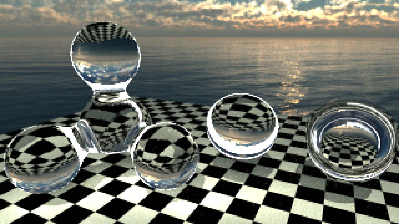
Have a look at Chapter 9.1.3 and 14.5.2 in the textbook for information. When finished you should, at a minimum, be able to show the "Refractive" scene model refracting its surroundings correctly (using Fresnel to calculate how much energy reflects and refracts), like the image shown.

To implement this following the material model stack we have, a good way would be to implement 2 new classes:

On one hand, you need a refractive BTDF class, which should receive the IoR upon creation, and which determines the refraction direction (or the total internal reflection direction) using the refraction formula. Start working on this by having this class as your only material, disregarding the rest of the stack.

On the other hand, when you want to put the refractive material into the stack, you will need a way to apply the transparency factor. For that, you should implement a Linear Blend class that acts between two BTDF, instead of two BSDF as we have right now. You can probably just copy most of the code into a new class (or make a template class, if you feel adventurous). Then you just have to replace the Diffuse object in the stack by a linear blend between the diffuse and the refracting materials.

Note: until now, we have been assuming that all rays come at a surface from outside, and leave the surface on the same side. You will need to make changes in the sample_wi method for the MicrofacetBRDF and DielectricBSDF to account for that (think what direction the wh points in each possible case), as well as in the Li function. You should take a look at the provided sameHemisphere function, it will be helpful in some of these cases.

You get more bonus points^(*) if you also calculate how energy is attenuated by transmittance. If you really want to show off, you could implement a proper rough refraction BRDF as described in, e.g., Microfacet Models for Refraction through Rough Surfaces by Walter et al.

Note: for simplicity, in the image above we are not properly accounting for the fresnel term when a light ray goes from a medium of higher index of refraction to a lower (air, in this case). The correct way is explained in Chapter 9.5.3 of the textbook.

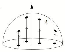
Area Lights

You path tracer currently only accounts for one point light source. Change that, so that it contains a number of area lights instead. Make sure to check out Chapter 10 in the textbook, as it provides all the information you should need to make this work. Note that having a large amount of point lights distributed over an area is not the same as a proper realistic area light, which has directionality baked in.

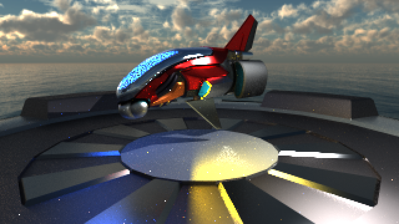
You will find a couple of structures that can help you with that in the Pathtracer.h file: There is a DiscLight class and a vector disc_lights that you can use for it. We have a couple of reference lights that you can enable by uncommenting the code in initialize() where they are added to the vector pathtracer::disc_lights, so if you implement it properly, the result with those should look like the image above. You can make new lights and change them however you want, but it will be easier for us to check that your implementation works if you show us how it looks with these two.

In the GUI you also have a checkbox named "Show Light Overlays", which should show you how all the lights in the scene look like.

You can look at Chapter 14 of the PBR Book for indications on how to use area lights. If you're feeling a bit ambitious you could let the light source have an arbitrary shape (by, e.g., loading an .obj model.). For extra bonus points^(*) you could add Multiple Importance Sampling (google or look in any raytracing book) to improve convergence.

Implement your own collision code

In this tutorial we have relied entirely on Intel's Embree library to do ray-tracing, but why let them have all the fun?

You could add code to support some custom parametric surfaces like, for example, spheres, elipsoids, cones, cillinders, boxes, or even Bézier surfaces. Having a couple of these working should be enough, but this can get as complex as you'd like. See Chapters 17 and 22.6 in the textbook for some details.

If you are very bored and feel like taking on a complex project with lots of potential headaches sounds like fun, you might even want to try rolling your own BVH. Using the simple interface described in embree.h, replace embree with your own acceleration structure and intersection routines. Anything better than just running through a list of triangles is good enough (But an Axis Aligned Bounding Box tree is probably a good choice). Chapters 19 and 22 in the textbook should contain information to get you started.

---

^(*) Any extra bonus points are strictly ornamental. The tutorials and projects are not graded.

---

When done, show your result to one of the assistants. Have the finished program running and be prepared to explain what you have done.