Biaffine graph-based dependency parsing
In this example, we will show the implementation of a graph-based dependency parser inspired by the work of Dozat and Manning (2017). We will train the parser on an English treebank from the Universal Dependencies collection. The parser can also be run interactively, so that you can see how example sentences are processed. To simplify matters, we put the evaluation step inside the neural network module; in a real-world parser, we would probably use a separate evaluation script.
You can run this example with other languages from UD, but in that case you will have to use a different set of word embeddings or train the model without word embeddings (which will also work).
The interactive part relies on the NLTK library for part-of-speech tagging and visualization and requires that you install this library, as well as graphviz if you want to draw the trees.
import torch
from torch import nn
import time
import torchtext
import numpy as np

import random

from collections import defaultdict, Counter

import matplotlib.pyplot as plt

%config InlineBackend.figure_format = 'retina'
plt.style.use('seaborn')
Reading the data
Let's first discuss the data and the way that it's formatted. We will use treebanks from the Universal Dependencies project.
We use the training and development sections of the English dataset. These files can be downloaded from the UD repository. You can read here about the format used in the UD project. Here is an example of a sentence in this format.
1       Now     now     ADV     RB      _                                 4       advmod  4:advmod
2       ,       ,       PUNCT   ,       _                                 4       punct   4:punct
3       people  people  NOUN    NNS     Number=Plur                       4       nsubj   4:nsubj
4       wonder  wonder  VERB    VBP     Mood=Ind|Tense=Pres|VerbForm=Fin  0       root    0:root
5       if      if      SCONJ   IN      _                                 9       mark    9:mark
6       Google  Google  PROPN   NNP     Number=Sing                       9       nsubj   9:nsubj
7       can     can     AUX     MD      VerbForm=Fin                      9       aux     9:aux
8       even    even    ADV     RB      _                                 9       advmod  9:advmod
9       survive survive VERB    VB      VerbForm=Inf                      4       ccomp   4:ccomp
10      .       .       PUNCT   .       _                                 4       punct   4:punct
To create torchtext Example objects, we extract columns corresponding to the word forms, part-of-speech tags, and head positions (columns 2, 5 and 7 respectively).
def read_data(corpus_file, datafields):
    with open(corpus_file, encoding='utf-8') as f:
        examples = []
        words = []
        postags = []
        heads = []
        for line in f:
            if line[0] == '#': # Skip comments.
                continue
            line = line.strip()
            if not line:
                # Blank line for the end of a sentence.
                examples.append(torchtext.data.Example.fromlist([words, postags, heads], datafields))
                words = []
                postags = []
                heads = []
            else:
                columns = line.split('\t')
                # Skip dummy tokens used in ellipsis constructions, and multiword tokens.
                if '.' in columns[0] or '-' in columns[0]:
                    continue
                words.append(columns[1])
                postags.append(columns[4])
                heads.append(int(columns[6]))
        return torchtext.data.Dataset(examples, datafields)
Defining the edge-factored dependency parser
We will now define the neural network model in the parser by Dozat and Manning. This model works as follows:
- for each token, we look up word and part-of-speech tag embeddings;
- we then apply a bidirectional, multi-layer recurrent neural network;
- finally, we use a biaffine neural network to compute the score for every potential edge in the sentence. Here is an overview figure from the Dozat and Manning (2017).
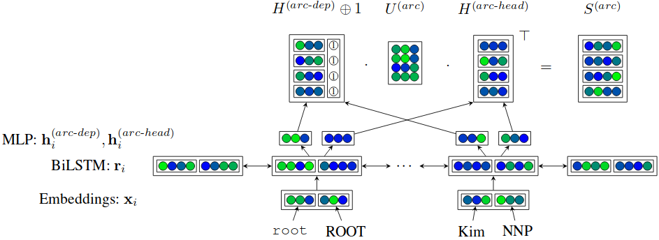
That is, we consider every word pair, and compute a score that will be high if the model thinks that those two words are connected in the dependency tree, and low otherwise.
Since this neural network is a bit larger than in our previous examples, we design it in a modular fashion. We implement the edge scorer and the sentence encoder as two separate modules (nn.Module). This means that they can be replaced more easily, for instance if we'd like to use an ELMo encoder instead of our straightforward LSTM, or if we'd like to use some other type of edge scorer (for instance, the one by Kiperwasser and Goldberg.)
class EdgeFactoredParser(nn.Module):

    def __init__(self, fields, word_emb_dim, pos_emb_dim,
                 rnn_size, rnn_depth, mlp_size, update_pretrained=False):
        super().__init__()

        word_field = fields[0][1]
        pos_field = fields[1][1]

        # Sentence encoder module.
        self.encoder = RNNEncoder(word_field, word_emb_dim, pos_field, pos_emb_dim, rnn_size, rnn_depth,
                                  update_pretrained)

        # Edge scoring module.
        self.edge_scorer = BiaffineEdgeScorer(2*rnn_size, mlp_size)

        # To deal with the padding positions later, we need to know the
        # encoding of the padding dummy word.
        self.pad_id = word_field.vocab.stoi[word_field.pad_token]

        # Loss function that we will use during training.
        self.loss = torch.nn.CrossEntropyLoss(reduction='none')

    def word_tag_dropout(self, words, postags, p_drop):
        # Randomly replace some of the positions in the word and postag tensors with a zero.
        # This solution is a bit hacky because we assume that zero corresponds to the "unknown" token.
        w_dropout_mask = (torch.rand(size=words.shape, device=words.device) > p_drop).long()
        p_dropout_mask = (torch.rand(size=words.shape, device=words.device) > p_drop).long()
        return words*w_dropout_mask, postags*p_dropout_mask

    def forward(self, words, postags, heads, evaluate=False):

        if self.training:
            # If we are training, apply the word/tag dropout to the word and tag tensors.
            words, postags = self.word_tag_dropout(words, postags, 0.25)

        encoded = self.encoder(words, postags)
        edge_scores = self.edge_scorer(encoded)

        # We don't want to evaluate the loss or attachment score for the positions
        # where we have a padding token. So we create a mask that will be zero for those
        # positions and one elsewhere.
        pad_mask = (words != self.pad_id).float()

        loss = self.compute_loss(edge_scores, heads, pad_mask)

        if evaluate:
            n_errors, n_tokens = self.evaluate(edge_scores, heads, pad_mask)
            return loss, n_errors, n_tokens
        else:
            return loss

    def compute_loss(self, edge_scores, heads, pad_mask):
        n_sentences, n_words, _ = edge_scores.shape
        edge_scores = edge_scores.view(n_sentences*n_words, n_words)
        heads = heads.view(n_sentences*n_words)
        pad_mask = pad_mask.view(n_sentences*n_words)
        loss = self.loss(edge_scores, heads)
        avg_loss = loss.dot(pad_mask) / pad_mask.sum()
        return avg_loss

    def evaluate(self, edge_scores, heads, pad_mask):
        n_sentences, n_words, _ = edge_scores.shape
        edge_scores = edge_scores.view(n_sentences*n_words, n_words)
        heads = heads.view(n_sentences*n_words)
        pad_mask = pad_mask.view(n_sentences*n_words)
        n_tokens = pad_mask.sum()
        predictions = edge_scores.argmax(dim=1)
        n_errors = (predictions != heads).float().dot(pad_mask)
        return n_errors.item(), n_tokens.item()

    def predict(self, words, postags):
        # This method is used to parse a sentence when the model has been trained.
        encoded = self.encoder(words, postags)
        edge_scores = self.edge_scorer(encoded)
        return edge_scores.argmax(dim=2)
Here is the implementation of the edge scoring part. We will follow the notation not from the original paper, but by their followup paper where the description is a bit clearer.
class BiaffineEdgeScorer(nn.Module):

    def __init__(self, rnn_size, mlp_size):
        super().__init__()

        mlp_activation = nn.ReLU()

        # The two MLPs that we apply to the RNN output before the biaffine scorer.
        self.head_mlp = nn.Sequential(nn.Linear(rnn_size, mlp_size), mlp_activation)
        self.dep_mlp = nn.Sequential(nn.Linear(rnn_size, mlp_size), mlp_activation)

        # Weights for the biaffine part of the model.
        self.W_arc = nn.Linear(mlp_size, mlp_size, bias=False)
        self.b_arc = nn.Linear(mlp_size, 1, bias=False)

    def forward(self, sentence_repr):

        # MLPs applied to the RNN output: equations 4 and 5 in the paper.
        H_arc_head = self.head_mlp(sentence_repr)
        H_arc_dep = self.dep_mlp(sentence_repr)

        # Computing the edge scores for all edges using the biaffine model.
        # This corresponds to equation 9 in the paper. For readability we implement this
        # in a step-by-step fashion.
        Hh_W = self.W_arc(H_arc_head)
        Hh_W_Ha = H_arc_dep.matmul(Hh_W.transpose(1, 2))
        Hh_b = self.b_arc(H_arc_head).transpose(1, 2)
        return Hh_W_Ha + Hh_b
And here is the sentence encoding part. This is a straightforward application of techniques we've seen in the past, with the small twist that we're using embeddings not only for the words but also the part-of-speech tags.
class RNNEncoder(nn.Module):

    def __init__(self, word_field, word_emb_dim, pos_field, pos_emb_dim, rnn_size, rnn_depth, update_pretrained):
        super().__init__()

        self.word_embedding = nn.Embedding(len(word_field.vocab), word_emb_dim)
        # If we're using pre-trained word embeddings, we need to copy them.
        if word_field.vocab.vectors is not None:
            self.word_embedding.weight = nn.Parameter(word_field.vocab.vectors,
                                                       requires_grad=update_pretrained)

        # POS-tag embeddings will always be trained from scratch.
        self.pos_embedding = nn.Embedding(len(pos_field.vocab), pos_emb_dim)

        self.rnn = nn.LSTM(input_size=word_emb_dim+pos_emb_dim, hidden_size=rnn_size, batch_first=True,
                          bidirectional=True, num_layers=rnn_depth)

    def forward(self, words, postags):
        # Look u
        word_emb = self.word_embedding(words)
        pos_emb = self.pos_embedding(postags)
        word_pos_emb = torch.cat([word_emb, pos_emb], dim=2)

        rnn_out, _ = self.rnn(word_pos_emb)

        return rnn_out
Training the full system
As usual, we build a main function that loads the dataset, creates a model, and goes through the training loop, and prints some diagnostics at the end. This is similar to our previous examples, so we'll leave it without comment.
While training, we print the unlabeled attachment score (UAS) evaluated on the validation set. We usually reach UAS levels of about 0.87-0.88 when we use this English dataset. (For other treebanks, the results might be very different, depending on the size of the treebank and the difficulty of the language.)
The only small quirk here is that the loss function computation and attachment evaluation have been put inside the forward step as we saw above, which means that we don't call call the loss function or any evaluation function here.
class DependencyParser:

    def __init__(self, lower=False):
        pad = '<pad>'
        self.WORD = torchtext.data.Field(init_token=pad, pad_token=pad, sequential=True,
                                         lower=lower, batch_first=True)
        self.POS = torchtext.data.Field(init_token=pad, pad_token=pad, sequential=True,
                                        batch_first=True)
        self.HEAD = torchtext.data.Field(init_token=0, pad_token=0, use_vocab=False, sequential=True,
                                         batch_first=True)
        self.fields = [('words', self.WORD), ('postags', self.POS), ('heads', self.HEAD)]
        self.device = 'cuda'


    def train(self):
        # Read training and validation data according to the predefined split.
        train_examples = read_data('data/en_ewt-ud-train.conllu', self.fields)
        val_examples = read_data('data/en_ewt-ud-dev.conllu', self.fields)

        # Load the pre-trained word embeddings that come with the torchtext library.
        use_pretrained = True
        if use_pretrained:
            print('We are using pre-trained word embeddings.')
            self.WORD.build_vocab(train_examples, vectors="glove.840B.300d")
        else:
            print('We are training word embeddings from scratch.')
            self.WORD.build_vocab(train_examples, max_size=10000)

        self.POS.build_vocab(train_examples)

        # Create one of the models defined above.
        self.model = EdgeFactoredParser(self.fields, word_emb_dim=300, pos_emb_dim=32,
                                        rnn_size=256, rnn_depth=3, mlp_size=256, update_pretrained=False)

        self.model.to(self.device)

        batch_size = 256

        train_iterator = torchtext.data.BucketIterator(
            train_examples,
            device=self.device,
            batch_size=batch_size,
            sort_key=lambda x: len(x.words),
            repeat=False,
            train=True,
            sort=True)

        val_iterator = torchtext.data.BucketIterator(
            val_examples,
            device=self.device,
            batch_size=batch_size,
            sort_key=lambda x: len(x.words),
            repeat=False,
            train=True,
            sort=True)

        train_batches = list(train_iterator)
        val_batches = list(val_iterator)

        # We use the betas recommended in the paper by Dozat and Manning. They also use
        # a learning rate cooldown, which we don't use here to keep things simple.
        optimizer = torch.optim.Adam(self.model.parameters(), betas=(0.9, 0.9), lr=0.005, weight_decay=1e-5)

        history = defaultdict(list)

        n_epochs = 30

        for i in range(1, n_epochs + 1):

            t0 = time.time()

            stats = Counter()

            self.model.train()
            for batch in train_batches:
                loss = self.model(batch.words, batch.postags, batch.heads)
                optimizer.zero_grad()
                loss.backward()
                optimizer.step()
                stats['train_loss'] += loss.item()

            train_loss = stats['train_loss'] / len(train_batches)
            history['train_loss'].append(train_loss)

            self.model.eval()
            with torch.no_grad():
                for batch in val_batches:
                    loss, n_err, n_tokens = self.model(batch.words, batch.postags, batch.heads, evaluate=True)
                    stats['val_loss'] += loss.item()
                    stats['val_n_tokens'] += n_tokens
                    stats['val_n_err'] += n_err

            val_loss = stats['val_loss'] / len(val_batches)
            uas = (stats['val_n_tokens']-stats['val_n_err'])/stats['val_n_tokens']
            history['val_loss'].append(val_loss)
            history['uas'].append(uas)

            t1 = time.time()
            print(f'Epoch {i}: train loss = {train_loss:.4f}, val loss = {val_loss:.4f}, UAS = {uas:.4f}, time = {t1-t0:.4f}')

        plt.plot(history['train_loss'])
        plt.plot(history['val_loss'])
        plt.plot(history['uas'])
        plt.legend(['training loss', 'validation loss', 'UAS'])

    def parse(self, sentences):
        # This method applies the trained model to a list of sentences.

        # First, create a torchtext Dataset containing the sentences to tag.
        examples = []
        for tagged_words in sentences:
            words = [w for w, _ in tagged_words]
            tags = [t for _, t in tagged_words]
            heads = [0]*len(words) # placeholder
            examples.append(torchtext.data.Example.fromlist([words, tags, heads], self.fields))
        dataset = torchtext.data.Dataset(examples, self.fields)

        iterator = torchtext.data.Iterator(
            dataset,
            device=self.device,
            batch_size=len(examples),
            repeat=False,
            train=False,
            sort=False)

        # Apply the trained model to the examples.
        out = []
        self.model.eval()
        with torch.no_grad():
            for batch in iterator:
                predicted = self.model.predict(batch.words, batch.postags)
                out.extend(predicted.cpu().numpy())
        return out


parser = DependencyParser()
parser.train()

Parsing example sentences
We will now show how to apply the dependency parser that we have trained to new sentences.
The parser requires the input to be tokenized and part-of-speech-tagged. We use the NLTK library, which you can install easily via pip or conda. Another alternative is to use spaCy here. If you want to try the parser with some other language, you will need to read the documentation for NLTK or spaCy to see if they include a tokenizer and tagger for that language, or you will have to rely on some other tools, or input the tokens and tags manually.
import nltk

# Download the tokenizer and part-of-speech tagger models if you haven't done it before.
# nltk.download('punkt')
# nltk.download('averaged_perceptron_tagger')
Here is an example how we can tokenize and tag a sentence using NLTK:
nltk.pos_tag(nltk.word_tokenize('The big dog lives in its little house.'))
We make a utility function that calls NLTK to tokenize and part-of-speech-tag the sentence, and then call the parser we trained above to find the head position for each word. We then print the words, tags and head positions as three separate columns.
def parse_sentence(sentence):
    tokenized = nltk.word_tokenize(sentence)
    tagged = nltk.pos_tag(tokenized)
    edges = parser.parse([tagged])[0]
    for i, ((word, tag), head) in enumerate(zip(tagged, edges[1:]), 1):
        print(f'{i:2} {word:10} {tag:4} {head}')
Here is the result of parsing an example sentence.
parse_sentence('The big dog lives in its little house.')
Drawing dependency trees
It's probably a bit more understandable to look at the parse trees visually than the column-based format above. NLTK also includes functionality to draw trees.
Drawing the trees in a notebook requires the installation of graphviz utilities. If you use pip to install packages, install this package; if you use conda, install this and this.
When running this example, I had to add the location of the dot utility to the PATH. This might or might not be necessary in your case.
# Put the directory where 'dot' is located first in the PATH.
import os
os.environ['PATH'] = '/opt/miniconda3/bin:' + os.environ['PATH']
def draw_sentence(sentence):
    tokenized = nltk.word_tokenize(sentence)
    tagged = nltk.pos_tag(tokenized)
    edges = parser.parse([tagged])[0]
    nltk_str = '\n'.join(f'{w} _ {h}' for ((w, _), h) in zip(tagged, edges[1:]))
    return nltk.DependencyGraph(nltk_str)
We can now draw a tree for the example we saw above.
draw_sentence('The big dog lives in its little house.')
Analysing some tricky cases
We will now consider some tricky types of syntactic constructions that are often difficult to process for automatic parsers. Please note that I've seen some variation here, and if you retrain the parser you may see a different result next time. (This probably means that the parser is quite uncertain for these cases, and the margin between the correct and incorrect attachment is small.)
Most automatic parsers have some difficulty attaching prepositional phrases (PP attachment). If we attach the PP incorrectly, the interpretation of the sentence can be a bit weird. For instance, in the sentence I ate spaghetti with tomato sauce, should we attach with tomato sauce to spaghetti (meaning that the thing that was eaten was "spaghetti with tomato sauce"), or to ate (meaning, probably, that I somehow used the tomato sauce as a tool when eating the spaghetti).
In this case, it seems that we happened to get the correct analysis (with tomato sauce is attached to the noun spaghetti), but as I mentioned you may get a different result if you retrain the model.
draw_sentence('I ate spaghetti with tomato sauce.')
If instead we consider the sentence I ate spaghetti with a friend, we'd like to see an attachment to the verb ate, because the friend is not a part of the dish, but a companion while we're eating.
Again, we seem to have attached the PP correctly in this case.
draw_sentence('I ate spaghetti with a friend.')
Another PP attachment example. The PP should be attached to the verb in this case.
draw_sentence('I saw a movie in Gothenburg.')
... and to the noun in this case. (So in this case we are attaching incorrectly.)
draw_sentence('I saw a movie from Gothenburg.')
Another tricky case for automatic parser is the attachment in coordinations: that is, clauses and phrases that are combined with coordinating conjunctions such as and or or.
Here is a sentence containing some coordinations. The analysis is not entirely correct: the two noun coordinations (spaghetti and sauce and beer and water) are connected correctly, but the attachment of the second verb phrase (to drink...) is incorrect. But again, you might get a different result when rerunning the notebook.
draw_sentence('I like to eat spaghetti and sauce and to drink beer and water.')
It is notable that in all the sentences above, the parser has produced trees even though we are not imposing a tree constraint. (For instance, we could use the Chu-Liu/Edmonds algorithm to make sure that we get a tree.)
However, if we input some nonsense words, it might happen that the parser gets confused and we get something that is not a tree. As you can see in this case, we have a cycle and there is no attachment to the dummy root token.
draw_sentence('ajk dfj akds jdfklj kdaj klaj jdf kjdfl ajdfs kalds this')
If we give a very complex sentence as an input, we might also (sometimes) see outputs that are not perfectly tree-shaped.
draw_sentence('Since the time of Caesar, the phrase Veni, vidi, vici has been used in military contexts; king Jan III of Poland alluded to it after the 17th-century Battle of Vienna, saying Venimus, Vidimus, Deus vicit ("We came, We saw, God conquered").')