Text classification using a word-based convolutional neural network
We continue to investigate text classification, this time using a convolutional neural network (CNN) instead of a CBoW representation. Our implementation is very close to that described by Kim (2014), except that we don't use any pre-trained word embeddings, which will be covered in the next lecture.
import torch
from torch import nn
import time
import torchtext

from collections import defaultdict

import matplotlib.pyplot as plt

%config InlineBackend.figure_format = 'retina'
plt.style.use('seaborn')
Declaring the neural network model
The only thing that differs from the CBoW notebook is that we are using a CNN as our classifier. The interesting components here are the following:
the convolutional layer:
nn.Conv1dthe pooling layer:
nn.AverageMaxPool1dornn.AverageAvgPool1d
We declare three different convolutional layers, which will be applied in parallel and whose outputs will be "glued" together in the forward method. The reason for this solution is to allow convolutional filters of different sizes. The structure is more or less identical to what we see in this figure:
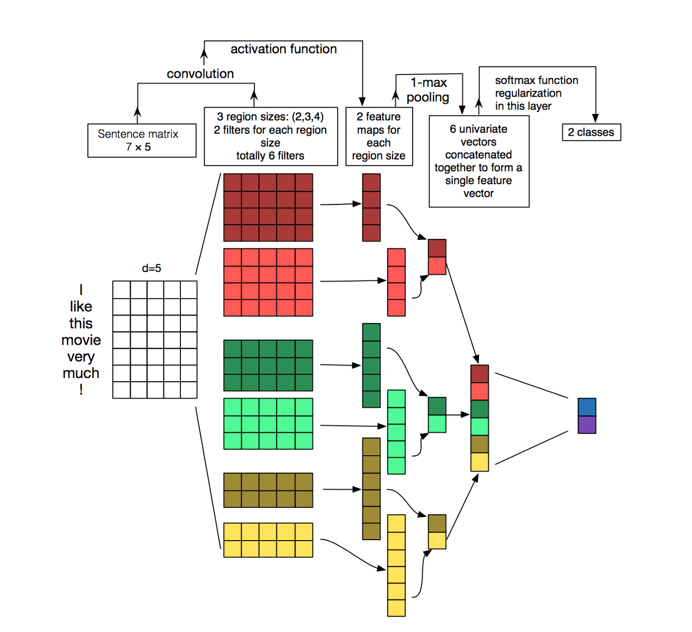 The steps are described in a more detailed fashion as comments in the code below.
class CNNTextClassifier(nn.Module):

    def __init__(self, text_field, class_field, emb_dim, conv_specs,
                 pooling='avg', dropout=0.1):
        super().__init__()

        # The inputs should mostly be self-explanatory, except the input conv_specs,
        # which is a list of pairs consisting of size and number of channels for each
        # convolutional layer, for instance [(2, 2), (3, 2), (4, 2)] corresponds to the figure.

        voc_size = len(text_field.vocab)
        n_classes = len(class_field.vocab)

        # Embedding layer.
        self.embedding = nn.Embedding(voc_size, emb_dim)

        # First convolutional layer.
        self.conv1 = nn.Conv1d(in_channels=emb_dim, out_channels=conv_specs[0][1], kernel_size=conv_specs[0][0])
        self.convs = [self.conv1]

        # Optionally, a second convolutional layer.
        if len(conv_specs) > 1:
            self.conv2 = nn.Conv1d(in_channels=emb_dim, out_channels=conv_specs[1][1], kernel_size=conv_specs[1][0])
            self.convs.append(self.conv2)

        # Optionally, a third convolutional layer.
        if len(conv_specs) > 2:
            self.conv3 = nn.Conv1d(in_channels=emb_dim, out_channels=conv_specs[2][1], kernel_size=conv_specs[2][0])
            self.convs.append(self.conv3)

        # A ReLU activation will be applied to the feature maps.
        self.activation = nn.ReLU()

        # For all feature maps, we'll apply a pooling operation over the whole sentence.
        # So we use an adaptive max or average pooling, with the number of regions set to 1.
        if pooling == 'avg':
            self.pooling = nn.AdaptiveAvgPool1d(1)
        else:
            self.pooling = nn.AdaptiveMaxPool1d(1)

        # Dropout for regularization.
        self.dropout = nn.Dropout(dropout)

        # To produce the output, a linear layer will be applied on the outputs from the pooling operation.
        n_channels = sum(nc for _, nc in conv_specs)
        self.top_layer = nn.Linear(n_channels, n_classes)

    def forward(self, texts):
        # The words in the documents are encoded as integers. The shape of the documents
        # tensor is (max_len, n_docs), where n_docs is the number of documents in this batch,
        # and max_len is the maximal length of a document in the batch.

        # First look up the embeddings for all the words in the documents.
        # The shape is now (max_len, n_docs, emb_dim).
        embedded = self.embedding(texts)

        # We need to "flip" the tensor so that it fits with the 1-dimensional convolution.
        # That is, the dimension over (the words) which we convolve needs to be the last one.
        # The shape is now (n_docs, emb_dim, max_len)
        embedded_t = embedded.permute(1,2,0)

        # We now apply the convolutional layers in parallel, and then the ReLU activation.
        # After these operations, each feature map now has the shape (n_docs, n_channels, max_len-size+1)
        # where n_channels is the number of "patterns" each convolutional layer looks for,
        # and size is the size of the convolutional filter.
        conv_maps = [ self.activation(conv(embedded_t)) for conv in self.convs ]

        # We apply the pooling operation. Since we pool over the whole sentence for each channel,
        # the results now have the shape (n_docs, n_channels, 1) for each convolutional filter.
        pooled = [ self.pooling(conv_map) for conv_map in conv_maps ]

        # We "glue" the results from all convolutional layers.
        # Shape: (n_docs, n_channels_in_total, 1)
        all_pooled = torch.cat(pooled, 1)

        # View the result as a two-dimensional tensor of shape (n_docs, n_channels_in_total)
        # The squeeze operation "hides" the third dimension of the tensor. This is equivalent
        # to calling all_pooled.view(n_docs, n_channels_in_total).
        all_pooled = all_pooled.squeeze(2)

        # Apply the dropout.
        all_pooled = self.dropout(all_pooled)

        # Finally, compute the output scores by applying a linear layer.
        # Shape: (n_docs, n_classes)
        scores = self.top_layer(all_pooled)

        return scores
Training the CNN text classifier
We train the CNN classifier and evaluate on the validation set. This code is identical to what we saw for CBoW, so I won't give detailed comments. The only differences are that we use the CNN classifier, that the learning rate is higher, and that we're using a lower number of epochs.
For the convolutional layers, we use a setup as in the figure above, with three 2-channel filters of size 2, 3, and 4 respectively. However, average pooling turned out to work better than max pooling in this case.
def read_data(corpus_file, datafields, label_column, doc_start):
    with open(corpus_file, encoding='utf-8') as f:
        examples = []
        for line in f:
            columns = line.strip().split(maxsplit=doc_start)
            doc = columns[-1]
            label = columns[label_column]
            examples.append(torchtext.data.Example.fromlist([doc, label], datafields))
    return torchtext.data.Dataset(examples, datafields)

def evaluate_validation(scores, loss_function, gold):
    guesses = scores.argmax(dim=1)
    n_correct = (guesses == gold).sum().item()
    return n_correct, loss_function(scores, gold).item()

def main():

    TEXT = torchtext.data.Field(sequential=True, tokenize=lambda x: x.split())
    LABEL = torchtext.data.LabelField(is_target=True)
    datafields = [('text', TEXT), ('label', LABEL)]

    corpus = 'amazon'
    if corpus == 'amazon':
        data = read_data('data/all_sentiment_shuffled.txt', datafields, label_column=1, doc_start=3)
        train, valid = data.split([0.8, 0.2])
    elif corpus == 'ag':
        train = read_data('data/ag_news.train', datafields, label_column=0, doc_start=2)
        valid = read_data('data/ag_news.test', datafields, label_column=0, doc_start=2)

    TEXT.build_vocab(train, max_size=10000)
    LABEL.build_vocab(train)

    corpus = 'amazon'

    # Declare the CNN classifier.
    model = CNNTextClassifier(TEXT, LABEL, emb_dim=32,
                              conv_specs=[(2, 2), (3, 2), (4, 2)],
                              pooling='avg', dropout=0.1)

    device = 'cuda'
    model.to(device)

    train_iterator = torchtext.data.BucketIterator(
        train,
        device=device,
        batch_size=128,
        sort_key=lambda x: len(x.text),
        repeat=False,
        train=True)

    valid_iterator = torchtext.data.Iterator(
        valid,
        device=device,
        batch_size=128,
        repeat=False,
        train=False,
        sort=False)

    loss_function = torch.nn.CrossEntropyLoss()
    optimizer = torch.optim.Adam(model.parameters(), lr=0.005)

    train_batches = list(train_iterator)
    valid_batches = list(valid_iterator)

    history = defaultdict(list)

    for i in range(20):

        t0 = time.time()

        loss_sum = 0
        n_batches = 0

        model.train()

        for batch in train_batches:
            scores = model(batch.text)
            loss = loss_function(scores, batch.label)

            optimizer.zero_grad()
            loss.backward()
            optimizer.step()

            loss_sum += loss.item()
            n_batches += 1

        train_loss = loss_sum / n_batches
        history['train_loss'].append(train_loss)

        n_correct = 0
        n_valid = len(valid)
        loss_sum = 0
        n_batches = 0

        model.eval()

        for batch in valid_batches:
            scores = model(batch.text)
            n_corr_batch, loss_batch = evaluate_validation(scores, loss_function, batch.label)
            loss_sum += loss_batch
            n_correct += n_corr_batch
            n_batches += 1
        val_acc = n_correct / n_valid
        val_loss = loss_sum / n_batches

        history['val_loss'].append(val_loss)
        history['val_acc'].append(val_acc)

        t1 = time.time()
        print(f'Epoch {i+1}: train loss = {train_loss:.4f}, val loss = {val_loss:.4f}, val acc: {val_acc:.4f}, time = {t1-t0:.4f}')

    plt.plot(history['train_loss'])
    plt.plot(history['val_loss'])
    plt.plot(history['val_acc'])
    plt.legend(['training loss', 'validation loss', 'validation accuracy'])

main()

The results will be a bit different each time due to random initialization. Typically, the accuracy is around 0.85, which is almost identical to what we got with the CBoW classifier. Probably, for this particular classification task there is no crucial need for a more complex classifier and we get quite far with a word-spotting approach.