Introduction

In this example we will spawn and simulate particles on the cpu which we, on each frame, will upload to the gpu. You will start by rendering simple fixed points from a fixed position. After that you will add velocity to those points, set the source at the exhaust of the ship, and finally use point sprites to render the particles as billboards with a texture.

Tasks

The system

In the files ParticleSystem.cpp and ParticleSystem.h we have provided a skeleton where it's up to you to fill in the blanks.

	void init_gpu_data();
	void spawn(Particle particle);
	void process_particles(float dt);
	void submit_to_gpu(const glm::mat4& viewMat);
	void kill(int id);

Before we start with the implementation of these functions, let's first take a look at the data structure for a particle.

    //The full particle state
    struct Particle {
        glm::vec3 pos;
        glm::vec3 velocity;
        float lifetime;
        float life_length;
    };

Here lifetime keeps track of how long the particle has been alive. lifelength is the maximum lifetime of the particle. When lifetime > lifelength, we consider the particle to be dead, and remove it (kill). The particle also has a position (the center of the particle) and a velocity. We keep a std::vector of the full states (particles), and a std::vector (gl_data_temp_buffer) with the reduced states (which will be uploaded to the gpu) on the CPU.

General procedure

The Particle struct contains all data we need for the simulation and you will also introduce a more compact struct which contains all we need for the rendering. For each frame we will do the following:

1. Eventually spawn particle(s) by calling spawn()
2. Process particles by calling process_particles()
   1. For each particle, remove if dead by calling kill()
   2. For each particle, update the state (see below)
3. Update the data on the gpu by calling submit_to_gpu()
   1. Update the vector of reduced states (gl_data_temp_buffer), from the full states (particles)
   2. Upload the data to the gpu
   3. Render the particles as point sprites

Gpu data

This section is important, it describes how the data will be sent to the GPU. You will probably need to refer to it several times during the project, so keep it in mind!

In order to render the particles you will need to create a vertex array object, to get the inputs to your vertex shader (see Tutorial 1). The input we need are the position and lifetime of the particle. Later we will render transparent particles, which we will need to sort depending on their view space depth, in order to get correct blending. Because of this we will do the view space transformation on the cpu and upload the already transformed positions. We will modify the lifetime at the same time, so that 0 corresponds to just spawned, and 1 corresponds to just about to die.

You don't need to upload anything here, just allocate enough memory to hold your data, i.e. call glBufferData with nullptr as the data pointer. Later you may want to make it so the buffer can hold as many particles as your particle system, but for now go ahead and allocate space for 100000 elements.

Hint: It is probably easiest to store the data as a vec4, where xyz is the view space position and w is the lifetime. If you want to experiment, once you have everything else working, you could try to use stride and offset to access the buffer as a vec3 and a float in the shader, instead of a vec4.

Extract the data we wish to upload

In order to extract the particle data we want to upload we will first copy the modified particle data from the system, here named particle_system. Since we have the GL (cpu) data in the member variable std::vector<glm::vec4> data; the last step (the sorting) is done like so:

    unsigned int num_active_particles = particles.size();
    /* Code for extracting data goes here */
    // sort particles with sort from c++ standard library
    std::sort(gl_data_temp_buffer.begin(), std::next(gl_data_temp_buffer.begin(), num_active_particles), 
        [](const vec4 &lhs, const vec4 &rhs){ return lhs.z < rhs.z; });

If you are not familiar with std::vector, here is some basic functionality:

1. vector.push_back() - append an element to the end of the vector
2. vector.pop_back() - remove an element at the end of the vector
3. vector.size() - returns the number of elements in the vector
4. vector.back() - returns the last element of the vector
5. vector.resize(int n) - Allocate space for n elements. OBS: size will be n and back will refer to the element at index n
6. Elements can be accessed as with arrays foo[i]

Note: The vector will grow dynamically if you use push_back.

Uploading data to the gpu

Uploading the data can be done by binding your buffer and then using glBufferSubData. This lets you upload a subset of the data, e.g. if your buffer holds 64 bytes, you can choose to upload only 8 if you wish.

Note:

1. The size of data we want to upload is the size of your GL data (in this case vec4) times the number of alive particles (num_active_particles).
2. The pointer to the data is acessed by data.data() (using &data[0] is equivalent except when data has 0 elements, in which case data.data() will return nullptr whereas &data[0] may crash by trying to access a null memory location).

Milestone

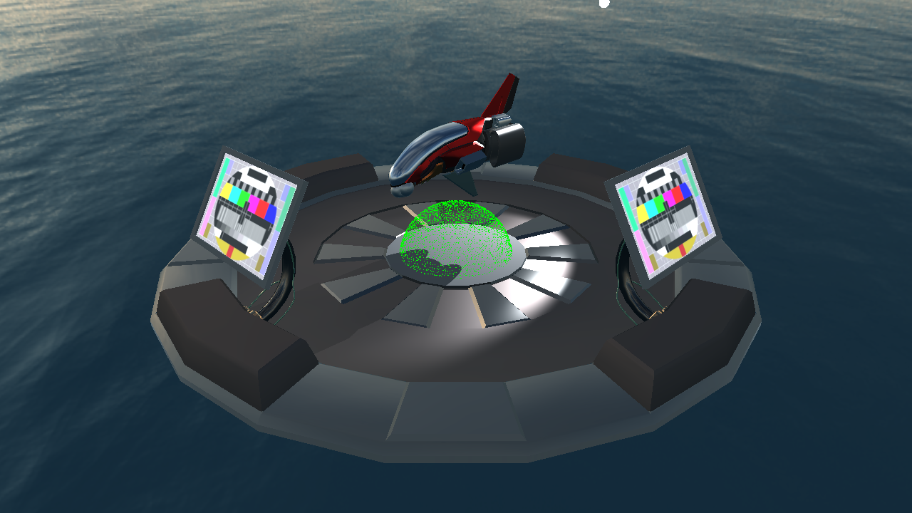
To see that we have got it working so far we can fill the GL (cpu) data with some values, upload it and render. To generate the positions we sample the surface of a sphere (http://mathworld.wolfram.com/SpherePointPicking.html), using the utility function labhelper::uniform_randf(float from, float to) which gernerates random floating point numbers in the specified interval.

    const float theta = labhelper::uniform_randf(0.f, 2.f * M_PI);
    const float u     = labhelper::uniform_randf(-1.f, 1.f);
    glm::vec3 pos     = glm::vec3(sqrt(1.f - u * u) * cosf(theta), u, sqrt(1.f - u * u) * sinf(theta));

Now, just scale the position by 10 to make the sphere larger, do the extraction and upload.
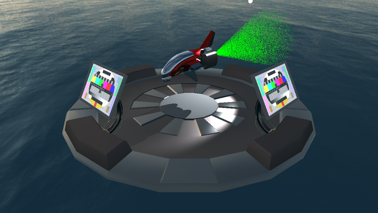
Bind a basic shader program where the vertex shader just does the projective transformation, and the fragment shader outputs the color green. Do not use the provided particle.vert and particle.frag shaders yet, as they won't work properly until the rest of the data is properly set up. Finally bind your VAO (vertex array object) and draw using glDrawArrays(GL_POINTS, 0, active_particles); where active_particles is the number of particles you just generated. You should have something like this:

Kill and spawn particles

Spawning a particle is fairly easy. Check if the number of elements is less than max_size and if so, push the element to the vector.

Killing a particle is quite straight forward as well. Simply copy or swap (you can use std::swap()) the last element to/with the element you want to kill, and then pop the last element of the std::vector. This way we are sure to only have alive particles in our vector. So go ahead and implement the kill and spawn functions. So you have a general idea, each of these two functions can be implemented with two to four lines of code.

Do the simulation!

So far we have only implemented the memory management of the system, so let's move on to actually do some simulation.

    void ParticleSystem::process_particles(float dt) {
        for (unsigned i = 0; i < particles.size(); ++i) {
            // Update alive particles!
        }
        for (unsigned i = 0; i < particles.size(); ++i) {
            // Kill dead particles!
        }
    }

The reason we have two loops here is that the way we kill particles doesn't allow for having both in the same loop. An added benefit is that the updating part is also much easier to be done in parallel.

Note: An alternative way of working could be to have 2 buffers, updating and copying only the alive particles from the previous frame to the second buffer, and swapping which one is used every frame. Each way has its pros and its cons, so we'll stick with our method for now.

Updating a particle is done by calculating the new position using the velocity and delta time (dt) as well as the lifetime (also using dt). If you desire, you could also update the velocity to simulate e.g. gravity, or air resistance.

Use the system

Now, try to use your particle system instead of generating the GL particles directly. Start by creating a large particle system in global scope.

    ParticleSystem particle_system(100000);

In the initialize() function you have to initialize the particle system so that the gpu memory can be allocated. Do this by calling

    particle_system.init_gpu_data();

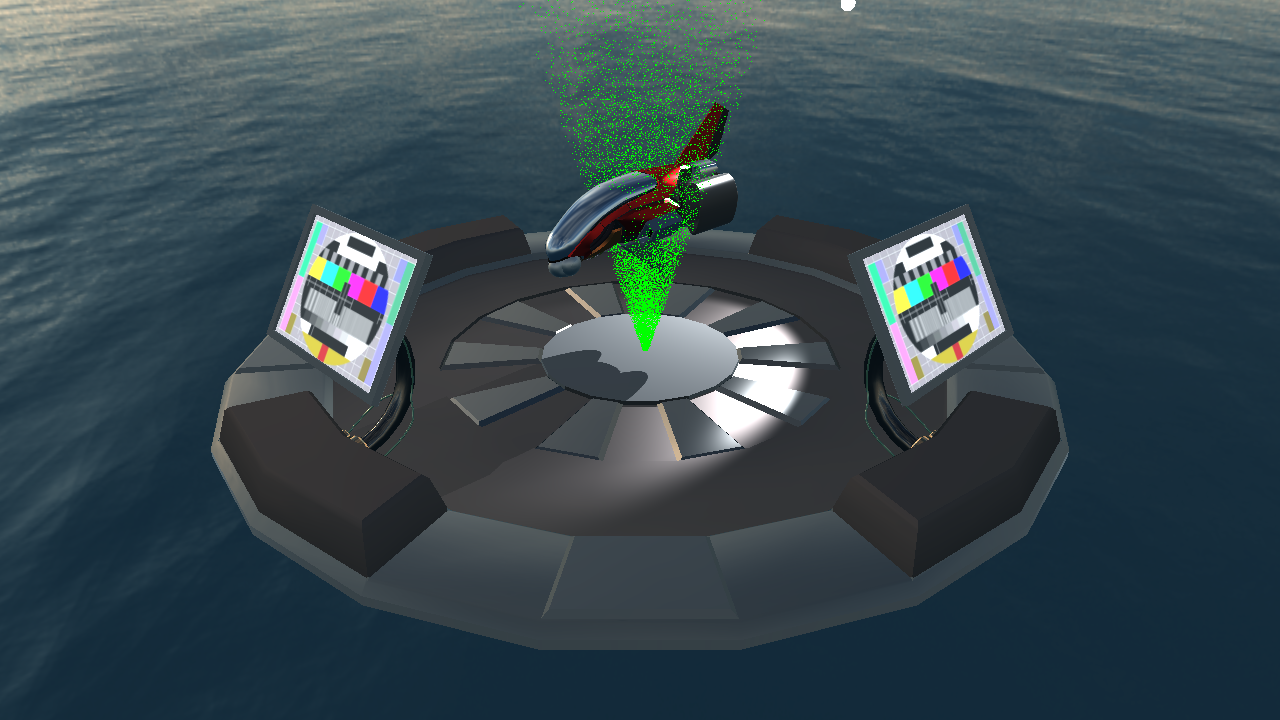
Every frame, create 64 particles where the initial position i zero, set the velocity equal to the position in your previous sphere sample (this creates random velocities radially outwards in different directions), lifetime as zero, and life_length to five. Do a simulation step, extract and upload.

To create a fountain, we can modify the sphere sample a bit by changing u:

    //const float u = labhelper::uniform_randf(-1.f, 1.f);
    const float u = labhelper::uniform_randf(0.95f, 1.f);

To change the axis of the fountain:

    //vec3(sqrt(1.f - u * u) * cosf(theta), u, sqrt(1.f - u * u) * sinf(theta))
    vec3(u, sqrt(1.f - u * u) * cosf(theta), sqrt(1.f - u * u) * sinf(theta))

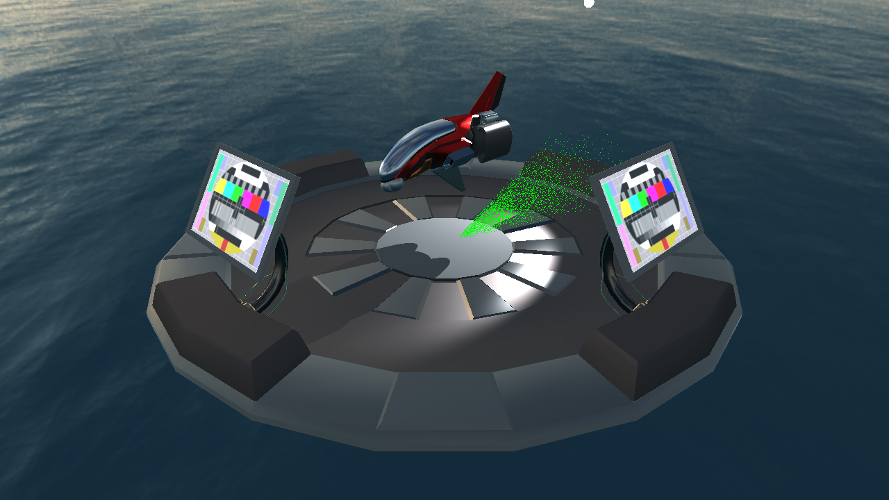
If we multiply the positions with the fighters modelmatrix they will be "attached" to the ship. Further try to offset the position (before the multiplication) so that they align to the exhaust.

Hint: ImGui::DragFloat3 may be of use here, letting you change a glm::vec3 of the initial position from the running application, instead of having to re-compile for each change.

Finally we can apply the rotation of the ship to the direction so that the particles always go out from the exhaust. Add keyboard controls for the ship, similarily to how you did in lab3 when you controlled the car (although, make use of glm's rotate() and translate()). Move the particle spawning code to the event handling as well, and use the rotation matrix applied to the direction to have a particle trail for the ship!

Note: The ship in this scene has the world x-axis as its forward vector, so you need to do some small modifications from the code in lab3.

Rendering pretty particles

We can use something called point sprites to render billboards with a texture. Now is a good time to use the provided shaders particle.vert and particle.frag. Also be sure to enable required functionality before the draw call:

    // Enable shader program point size modulation.
    glEnable(GL_PROGRAM_POINT_SIZE);
    // Enable blending.
    glEnable(GL_BLEND);
    glBlendFunc(GL_SRC_ALPHA, GL_ONE_MINUS_SRC_ALPHA);

And disable GL_BLEND and GL_PROGRAM_POINT_SIZE after rendering the particle data.

This will allow us to:

1. Modify the point size from within the shader.
2. Give uv-coordinates for the point.
3. Enable blending

Load explosion.png and bind it to unit 0. Lastly, add these lines of code when rendering the particles to allow us to properly scale the points.

    labhelper::setUniformSlow(particleProgram, "screen_x", float(windowWidth));
    labhelper::setUniformSlow(particleProgram, "screen_y", float(windowHeight));

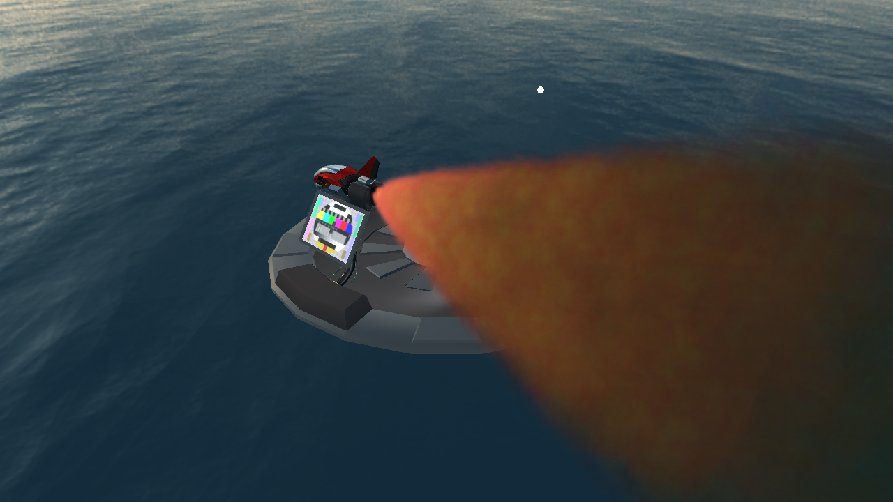
Now, drive around with your blazingly fast space ship!

What's next? [Optional]

Now you have a particle system working for the main engine, but what if you wanted to have one for a second ship? or for the other engines?

What would it take to have multiple particle systems generating particles at different points and towards different directions?

And what about if you want different kinds of particles? The way we fade out the particles and change their size as they age is a bit specific to the exhaust of the engine, but don't worry too much about that. More complex particle systems tend to have parameters to change these behaviours.

Think on how you could solve these problems, and give it a try if you feel intrepid.

---

When done, show your result to one of the assistants. Have the finished program running and be prepared to explain what you have done.