Introduction

Back in Lab 4, when we implemented physically-based illumination, we approximated global illumination and reflections with some precomputed images derived from the environment map.

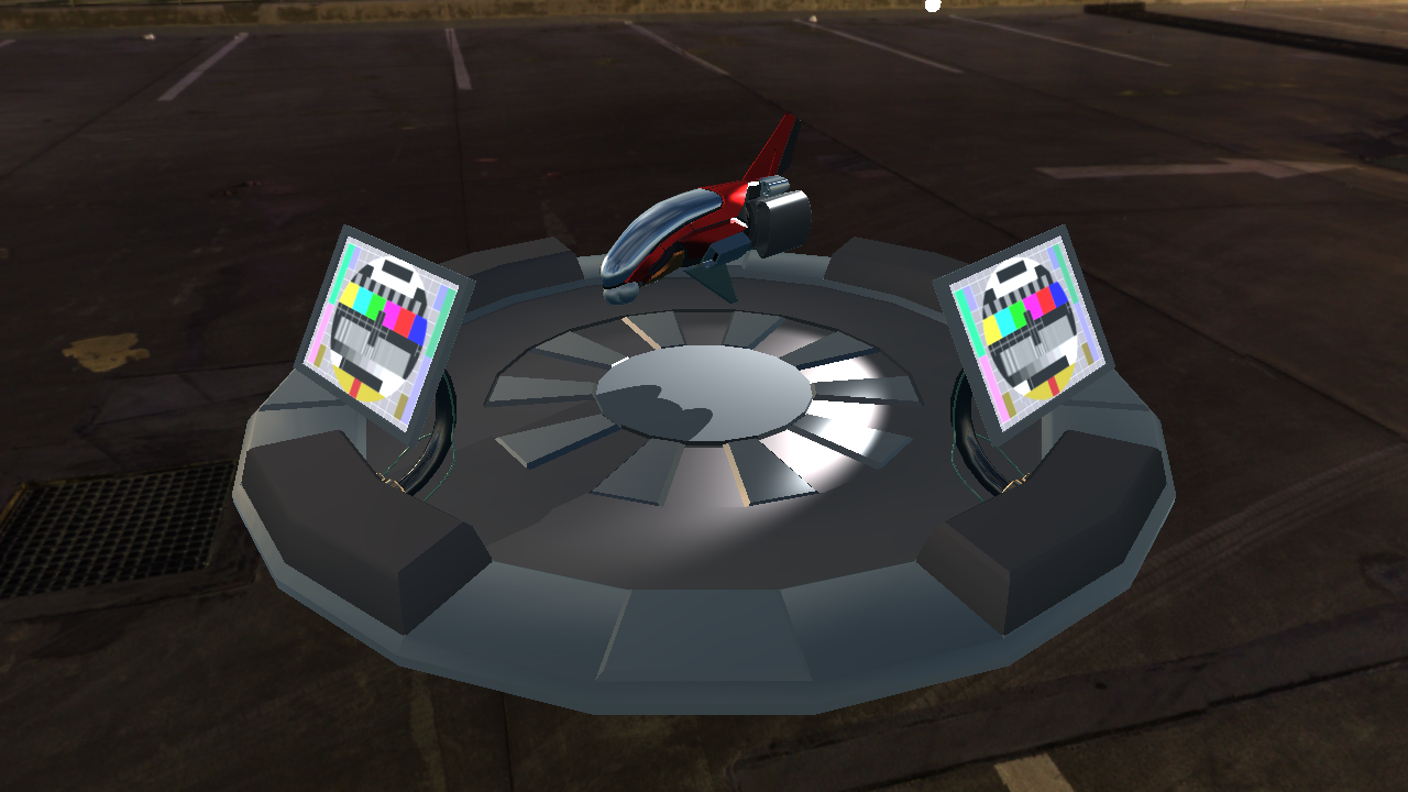
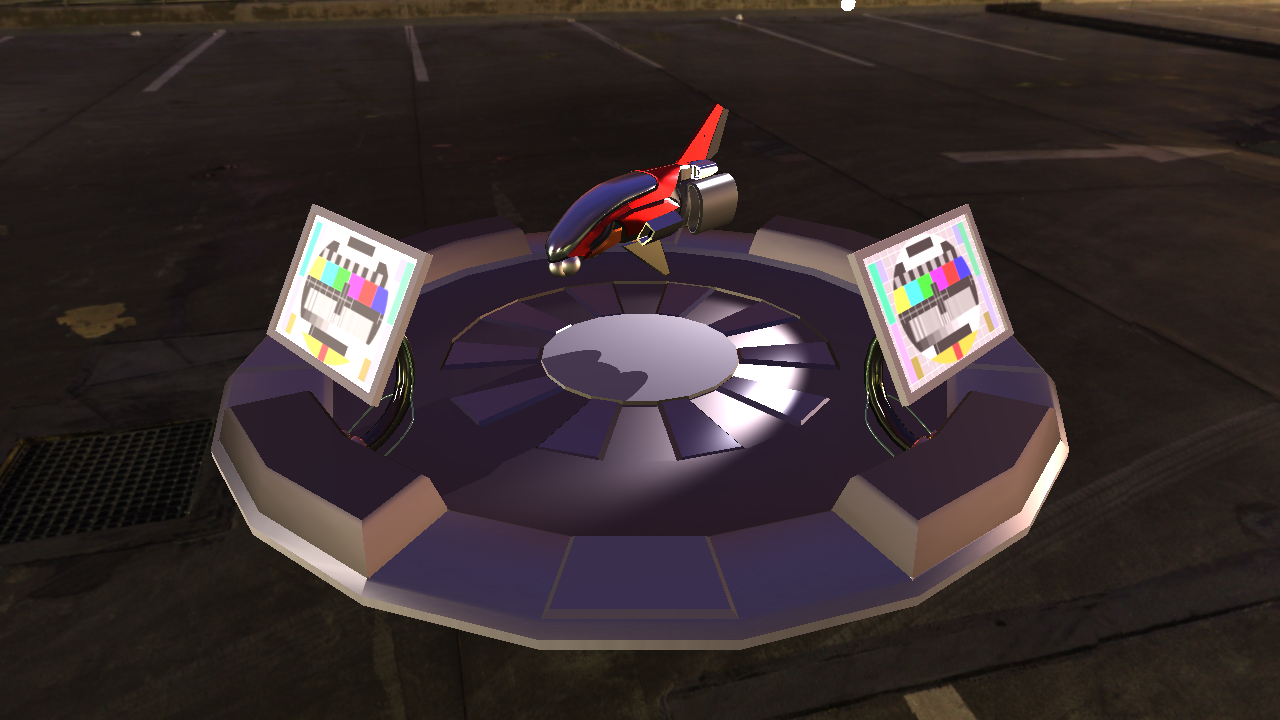
So if we wanted to use a different backgrond, only changing the environment map would not be enough, we would also need the proper images for the irradiance map and reflectivity map. Otherwise, the 3D objects would look out of place and with the wrong reflections:

In this project, you will implement a system that can precompute the images needed for this. In essence, what these images contain is the integral of the incoming light for a specific direction and material, that can be used as an approximation of what would be raytraced in the real scene.

Let's recall how the light we see reflected at a point is calculated. It follows the following formula:

where \(L_o(\omega_o)\) is the light leaving the point (and going to the eye, in this case), \(\int_{\Omega}{}\) represents the integral over all the possible directions (i.e. the integral over the surface of the unit sphere), \(f(\omega_i, \omega_o)\) is the BRDF for the material of the point for the given directions, \(n\) is the normal of the surface at the point, and \(L_i(\omega_i)\) is the light coming at the point from the direction \(\omega_i\).

This, as mentioned, is an integral over the whole sphere, which would include reflections coming from outside of the material, as well as refracted light coming from inside. We are only interested in opaque materials, so the only refractions we get are from the scattering of the light at the surface of the material (similar to subsurface scattering), which we model as diffuse light. We can then divide this sphere of incoming light in two hemispheres, the one along the normal, which will handle the reflections, and the one opposite the normal, which we will be handled as diffuse illumination:

Here \(c\) is the color of the material.

The \(F(\omega_i)\) is the Fresnel term, which determines the amount of light that would be reflected or absorbed/refracted/scattered by the surface, and depends on the material properties.

Irradiance map

Let's look first at the part concerning the diffuse illumination (the second integral in the last formula):

The Fresnel term depends on the material, but we can approximate it away by taking into account that the diffuse term is only going to be applied to dielectric materials (metals absorb almost all the light that is not reflected, while dielectrics scatter that light after tinting it), and that those usually have very low \(F_0\) values, which means that the value of \((1-F)\) will be very close to 1, and at grazing angles, where it varies the most, we don't really care that much because the cosine term (coming from the dot product) will make it count very little anyway.

Since the BRDF is constant, and we can wish the \(1-F\) away, this integral only depends on the incoming directions, and we can precompute that into a single image where every pixel represents a direction for \(n\) without needing approximations*.

(*): Except, of course, that we won't be able to take the occlusions by objects on the scene into account. But as long as we are lighting only a sphere floating in the void, we are golden!

So the final formula for this part, after taking the simplifications into account, becomes

Reflectivity map

This one is trickier, because the model we use for the BRDF is much more complex. The corresponding part of the integral here would extend to:

In this case, we will approximate \(F(\omega_i)\) by calculating it only for the perfect reflection direction, which is a function of \(\omega_o\) and \(n\), so it becomes constant with respect to \(\omega_i\) and so we can leave it out of the integral.

On the other hand, \(D(\omega_i, \omega_o)\) varies a lot depending on the material properties, so we can't really hope to simplify that away. Specifically, for rough materials, \(D\) will have a much wider angle of directions it takes light from, compared to a smooth/shiny material, which will have reflections in a very reduced set of directions.

To account for that, then, we will generate images for this term at different roughness values, and sample from the correct one during runtime. But that still leaves a dependency to knowing \(\omega_o\) when calculating the value for the term. What we will do, in this case, is precompute the values of the integral for \(\omega_o = n\).

The formula then becomes

Notice that the divisor is in part cancelled by the dot product that we had in the integral, and also because \(n \cdot n = 1\), and the \(G\) term gets simplified in a similar way thanks to us choosing \(\omega_o = n\).

Tasks

First off, we need a shader for each integral we want to calculate.

We are going to use Monte Carlo integration to approximate the integral's value; this method is explained in much more detail in the pathtracing project, but it boils down to taking samples of the function in random directions and averaging them together, accounting for the probability of taking each of the samples.

So, each frame, the shaders will take a few randomised samples of the function, account for the probability of each sample, and accumulate them in some buffer.

To accumulate them, we are going to trick the GPU into doing the calculation for us, taking advantage of the alpha blending functionality of the shading pipeline.

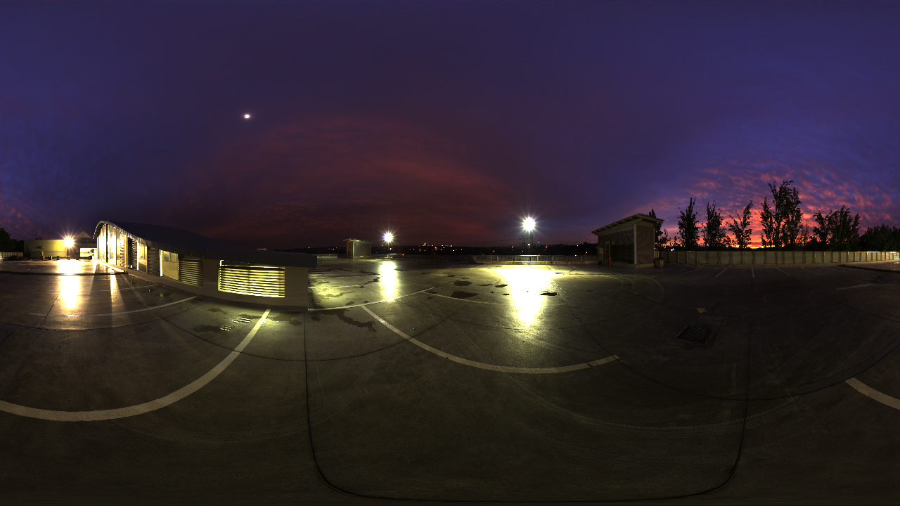
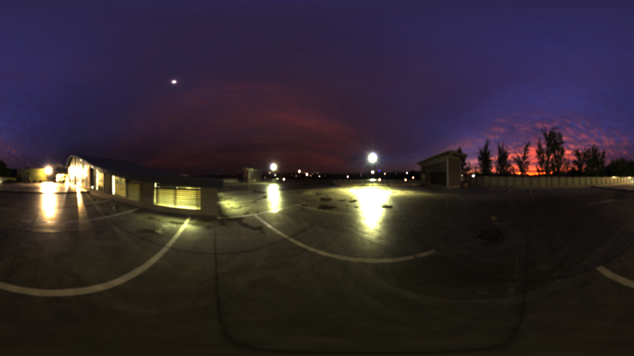
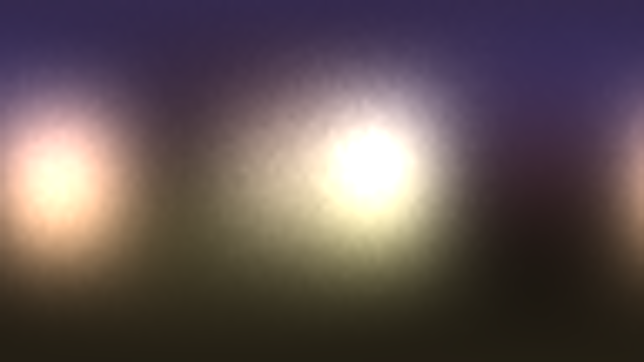
You can test things with the environment map found in scenes/envmaps/night.hdr, which looks like this:

Getting started

You will find a couple of shader files already created for this assignment: irradianceMap.frag and reflectivityMap.frag, which go together with the fullscreenQuad.vert. We have populated those with some functions to create random values that you will need later.

You can then visualize the created textures by rendering them at fullscreen with the ../pathtracer/copyTexture.vert and .frag shader.

Create a couple of global variables we will use to count the samples we take:

int numReflectivitySamplesTaken = 0;
int numReflectivitySamplesPerFrame = 16;

You will need to send both of these values to the irradianceMap and reflectivityMap shaders. The reflectivityMap also takes the roughness value (a value from 0 to 1). If you have, say, 7 roughness levels, then the values sent should be 0.5, 1.5, ... 6.5.

Accumulating the partial results

Start by creating a framebuffer for each of the images we want to create. That will be one for the irradiance map, and N for the reflectivity maps, one for each value of the roughness we want to have. Have them all have an aspect ratio of 2 (height = 2 * width) and, since the rougher the material is, the blurrier the image would look, have each level of the reflectivity be half the size of the previous one (say your first level is 1024 in width, the second will be 512, the third 256, and so on).

You will render onto all of these buffers every frame but, to be able to see what's going on, we recommend that you implement a way to select one of them to be copied to the screen with the copyTexture shader. A way would be to add a set of ImGui::RadioButton controls (see how that's implemented in lab 6 for an example), and a global index that selects which of the images to render.

We want to accumulate thousands of samples, so we will need too have some precision in these buffers for this to work properly, so we want them to be 32bit floats for each channel. The FboInfo class in the project can be made to use 32 bit floats by setting the variable colorTargetType of each buffer to GL_RGBA32F before calling resize().

Once you have the buffers created, you can render to them. Render to the irradiance map buffer with the corresponding shader, and loop through the reflectivity map buffers and render to each of them with the corresponding shader. Remember to set the viewport adequately every time.

If you render these images to the screen, you will see some random noise.

In this case, since we want to accumulate, you should not clear these framebuffers every frame. Instead, clear them only when numReflectivitySamplesTaken is 0.

Now, to accumulate the values, consider that we have an accumulation buffer with value \(a\) obtained from \(N\) samples, and the we are rendering a value \(b\) obtained from getting \(M\) samples each frame. The next frame, that buffer will have \(N+M\) samples, and so on. So basically, we can do a weighted average of the two values like \(\frac{a M + b N}{M + N} = a (1 - \frac{N}{M + N}) + b \frac{N}{M + N}\).

To do that, we will use, as said, the blending functionality. If you look at the possible values that the blend function can have, the ones that interests us right now are the CONSTANT_ALPHA ones. These take a constant value that we set from C, and use that instead of any value that the alpha channel might have. If we set this constant value to the factor \(\frac{N}{M + N}\), then we will get the last formula from above. You can use the code below:

glBlendFuncSeparate(GL_CONSTANT_ALPHA, GL_ONE_MINUS_CONSTANT_ALPHA, GL_ZERO, GL_ONE);
glBlendColor(0, 0, 0, float(numReflectivitySamplesPerFrame)
                        / float(numReflectivitySamplesTaken + numReflectivitySamplesPerFrame));

Make sure to enable blending.

Once this is done, if you render one of these images to the screen, you should see it start as random noise, but average to grey over time.

Before moving on, make sure also bind the environment map image before rendering onto all these surfaces, since we will sample from that.

Irradiance

This one is very simple.

Start by calculating the direction that the current pixel corresponds to. We will take this to be the normal in the integral formula. You can use the following to obtain spherical coordinates from the X and Y directions:

Create a vec4 variable where you can accumulate the samples from the environment map. Then do a loop from 0 to num_samples. Each iteration, you will sample a randomised direction, sample the environment map with that direction, and accumulate it to the vec4 variable from before. After the loop is done, set the fragmentColor to this value, divided by the number of samples you have taken.

Now let's go through what we need to integrate:

The way Monte Carlo sampling works is that we take a sample value from a random input value, and divide that by the probability of the random value. So if we take uniform samples over the hemisphere, we would evaluate them on the integral, and divide the result of that by the probability of each sample, which would be the constant \(2 \pi\). But we can be smarter here, since the values close to the normal direction will be more relevant thanks to the dot product, taking more samples in those directions will lead to faster convergence. More specifically, if we take them in a way that the probability follows a cosine distribution relative to the normal, the cosine in the integral will cancel out, and we can just accumulate the values sampled from the environment map.

So, use the sampleHemisphereCosine to get a sample in tangent space. Then, convert from tangent space to world space with the matrix you get from the tangentSpace function passing the normal direction you calculated from the pixel position. Now, convert this direction to spherical coordinates, and use them to sample from the environment map.

To account for the \(\pi\) factor from the integral, multiply the average obtained by it when setting it to the fragmentColor.

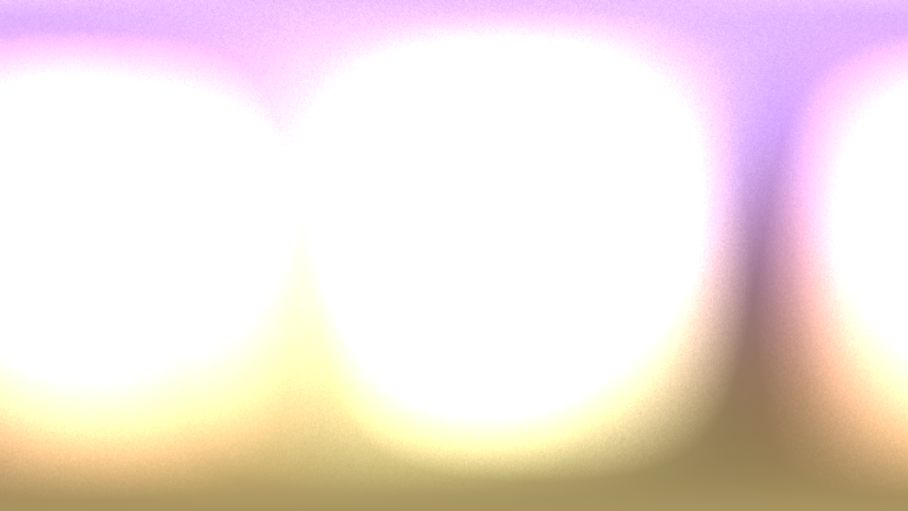
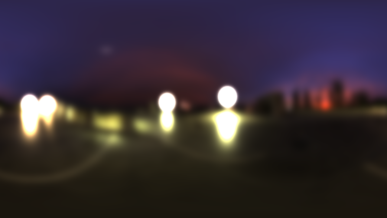
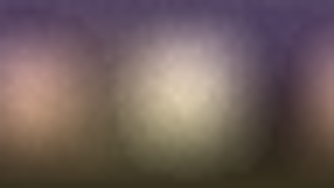
When rendering this, it should produce an image similar to the following:

Reflectivity

The basic procedure here will be similar as before, obtain a direction from the pixel position, and iterate and accumulate samples. What changes is the function we use to calculate the sample direction, as well as the factor multiplying the sample value.

First off, we need to calculate the shininess value from the roughness. That can be done with the following formula:

The way we will sample will be the same as is used in the pathtracer project. Refer to that if you want a more detailed explanation.

Now we will start by sampling a normal for the microfacet surface, then we will reflect our view direction on it, and that will give us the direction where the light came from, which we can use to sample the environment map.

Start by obtaining some random numbers from the random function, using the index for the current sample as input:

vec3 r = rand3f(float(samples_taken + i));

Then we use that to calculate the theta and phi of the microfacet surface:

Keep the cosine and sine term in separate variables, as we will use them as they are; you can now calculate the probability of having sampled this normal with the following:

If the value of the PDF is too low (less than, for example, 0.0001) skip the sample (just continue to the next iteration of the loop).

Now, use these values to calculate the tangent-space direction of this normal, bring it to world-space (multiply by the tangentSpace(n)) and reflect n (what we use as wi) around it, to obtain wo (remember, reflect does the negative of what one expects in these cases).

This will be the direction you need to sample from the environment map. But the way that it's sampled, there's some cases in which this could be a direction behind the surface defined by n, so check that dot(wo, n) is greater than 0. If it's not, then also skip this sample with continue.

Convert this world-space wo and sample the texture.

Let's also calculate the \(D\) term:

Before we calculated the PDF of sampling wh, but what we really need is the PDF of sampling the reflected wo. You can obtain that with:

Finally, the value to accumulate for this sample is:

Now, notice that we have possibly skipped some samples, so when averaging the accumulated values, you need to account for that. You will need a variable that counts how many good samples you have really obtained, and divide by that in the end. This has the caveat that there's the possibility that all the samples will be skipped, and would end up dividing by 0. To avoid that, make the loop continue until either the amount of samples to take is taken, or while we still have 0 samples.

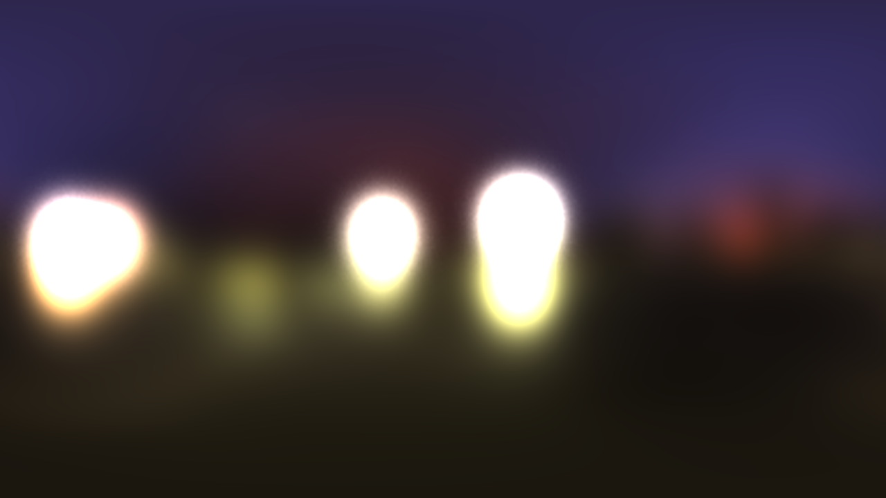
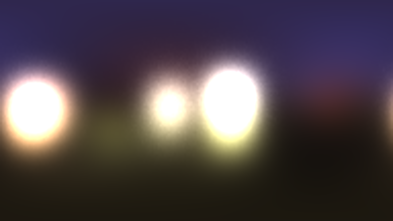
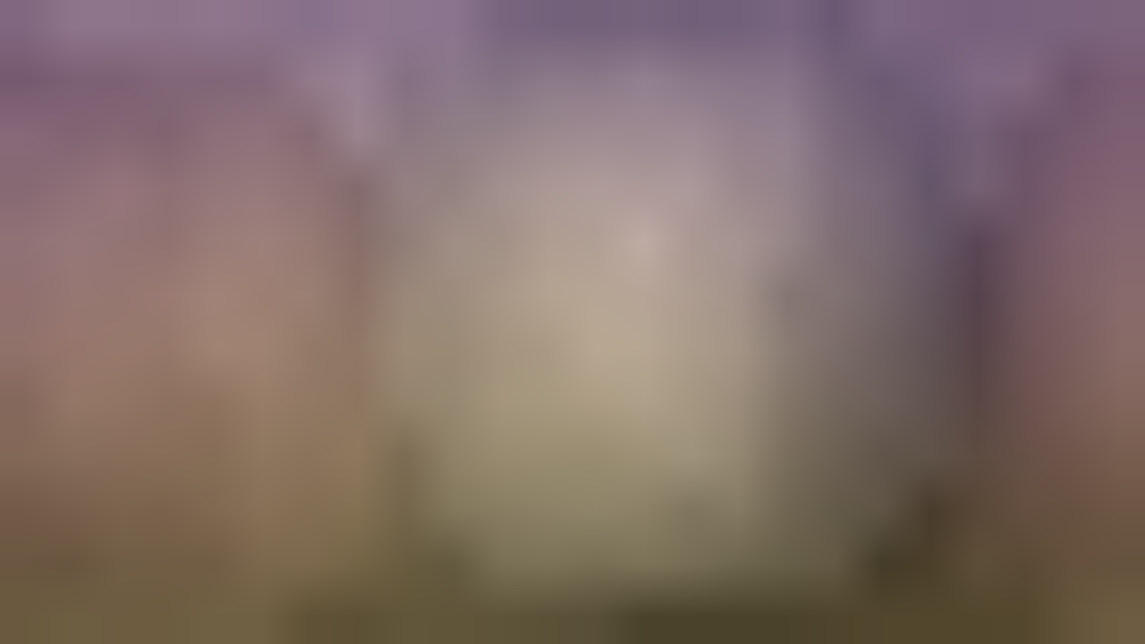
Once this is finished, you should end up having a set of images similar to this, after taking a several thousand samples:

Applying the environment maps to the scene

Now you have two options: you can either save the computed images to file and load them to the scene, or you can update the textures directly with the computed images from inside the application.

To save them to file, add a button to the GUI that, whenever pressed, calls the function labhelper::saveHdrTexture(filename, texture_id) for each of the computed textures. This will save both a .hdr texture and a tonemapped .png texture so you can see the resulting image (you might have noticed there's not many image viewing programs that deal with hdr images). The tonemapped png will not match what you see in the application when rendering because it's tonemapped using Reinhard's operator.

To update the images instead, you need to copy the contents of each framebuffer to the textures used for the irradiance and reflectivity maps. You can probably do it every frame without losing a lot of performance, and that could let you see the result of the computations in real time in the actual scene.

For this, you will neeed to first set the target texture sizes to the same as the framebuffers (you can use glTexImage2D sending NULL as the last parameter), and then every frame call glCopyTexSubImage2D(). Notice that the second argument to this function is the "level". That means the mipmap level, which you should take into account when updating the reflectivity map texture, since that one uses a mipmap the different roughness levels.

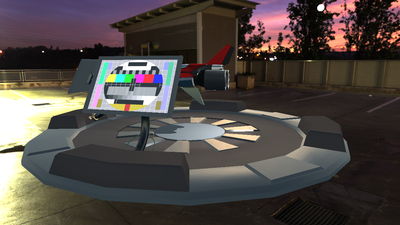
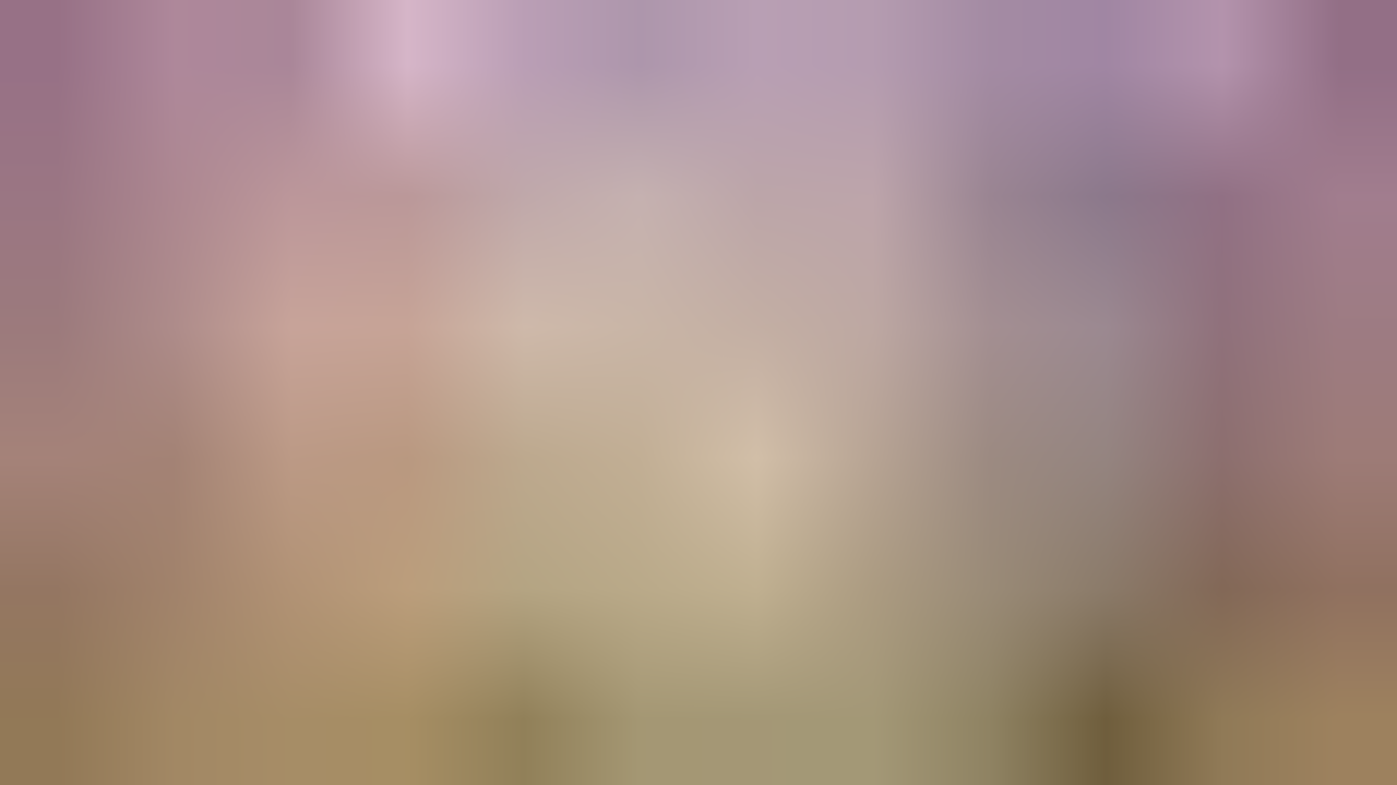
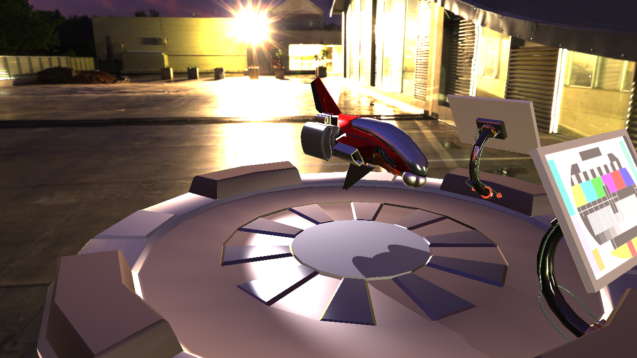
Now your scene should look something like this:

If you search the internet for something like "hdri environment map", you will find a bunch of other free options to try different things as a replacement environment map.

Optional

Improving randomness

To generate random numbers, we used one of the hashing algorithms that have better performance in the paper by M. Jarzynski and M. Olano¹, but other options could be used instead.

A good idea that could improve convergence times would be using a low-discrepancy function; a very straightforward one to implement is the family of functions based on the metallic numbers² (golden ratio et al.).

If you try to just use those as they are, you will probably run into the issue of not having enough randomness, having the sequence reach a point where you have a lot of patterning and there's no further improvement. There are options to fix that, for example by using fixed-point arithmetic instead of floating point when calculating the random numbers (since we only care about what's in the range from 0-1, you can have the whole integer value represent the right side of the decimal point, with an implicit 0 on the left).

Give this a try if you want, and see if you get better results with it.

---

When done, show your result to one of the assistants. Have the finished program running and be prepared to explain what you have done.