Introduction

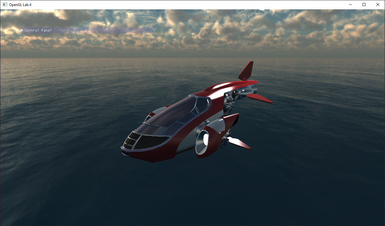
In this tutorial, we will learn to write a physically based shader. Compile and run the project, and you will see that we have supplied some starting code for you:

Start State

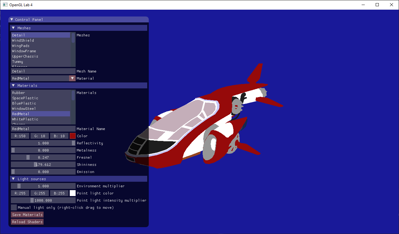
The code reads an .obj file with an associated material (.mtl) file. We have also added a GUI (in the function gui()) where you can change the properties of the materials. Currently, the only property that your shader respects is the color attribute. Go through the lab4_main.cpp file and make sure you understand what's going on. There shouldn't be anything really new to you here. Ask an assistant if some part confuses you.

Understand the GUI

Note:
In this tutorial, you can press the "reload shaders" button to recompile your shaders without restarting your program.
Start by selecting the ship's chassi ("UpperChassi") from the list in the "Meshes" category. It is currently set to use the "RedMetal" material. Change this to one of the unused materials instead. This will also select the unused material in the list of materials in the next category. Now change the name of that material to "BlueMetal", and change the color to be blue. If you like the result you can press the "Save Materials" button to save it.

Part 1: Direct illumination

Now take a look at the fragment shader used to render the spaceship. The only new thing in here so far is the uniforms that tell you about the current material:
///////////////////////////////////////////////////////////////////////////////
// Material
///////////////////////////////////////////////////////////////////////////////
uniform vec3 material_color;
uniform float material_reflectivity;
uniform float material_metalness;
uniform float material_fresnel;
uniform float material_shinyness;
uniform float material_emission;
These values correspond exactly to the values that you can set for each material in the GUI.

Have a look now at the main() function. So far it does not do very much, and it's up to you to fill it in. Let's start with calculating a proper diffuse reflection.

Diffuse term.

Before we can get anything real out of calculateDirectIllumination(), we need to figure out its input parameters
///////////////////////////////////////////////////////////////////////////
// Task 1.1 - Fill in the outgoing direction, wo, and the normal, n. Both
//            shall be normalized vectors in view-space.
///////////////////////////////////////////////////////////////////////////
vec3 wo = vec3(0.0);
vec3 n = vec3(0.0);
The BRDF:
Later in the course, you will learn about the BRDF (Bidirectional Reflectance Distribution Function), but we will use the term already in this lab. The BRDF is a function that says how much of the incoming radiance (light) from a specific direction $\omega_i$ is reflected some outgoing direction $\omega_o$.
Fill in the correct values for $ w_o $, the outgoing direction, and $ n $, the normal. Both of these should be normalized and in view-space.

Hint: In viewspace, the cameras position is $(0,0,0)$.

Then, in calculateDirectIllumination(), we need to calculate the incoming radiance from the light,

$d = $ distance from fragment to light source
$ L_i = $ point_light_intensity_multiplier * point_light_color * $ \frac{1}{d^2} $

Note:
We divide the color of the material with $\pi$ to get the diffuse BRDF.
We multiply the incoming radiance with $(n\cdot \omega_i)$ to get the incoming irradiance
and the direction from the fragment to the light, $w_i$ (in view space). Time for an early exit! If $n \cdot w_i <= 0$, then the light is incoming from the other side of the triangle, so this side will not be lit at all. In that case, your direct illumination code should just return black.

Finally, we can calculate the reflected light for a perfectly diffuse surface:
diffuse_term = material_color * $ \frac{1.0}{\pi}$ * $|n \cdot w_i|$ * $L_i$

Now return the diffuse term and look at the result:

Task 1

Try changing the light intensity and color and make sure your illumination changes. You are now rendering a perfectly diffuse spaceship. Let's add another simple thing. The enginges should shine whether they are lit or not, since they emit light themselves. Find where in the shader the emission term is added, and set emission to 
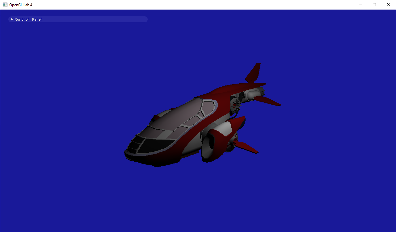
material_emission * material_color

Task 1.4

Change Scene.

Before we go on, let's switch to a different scene. In 
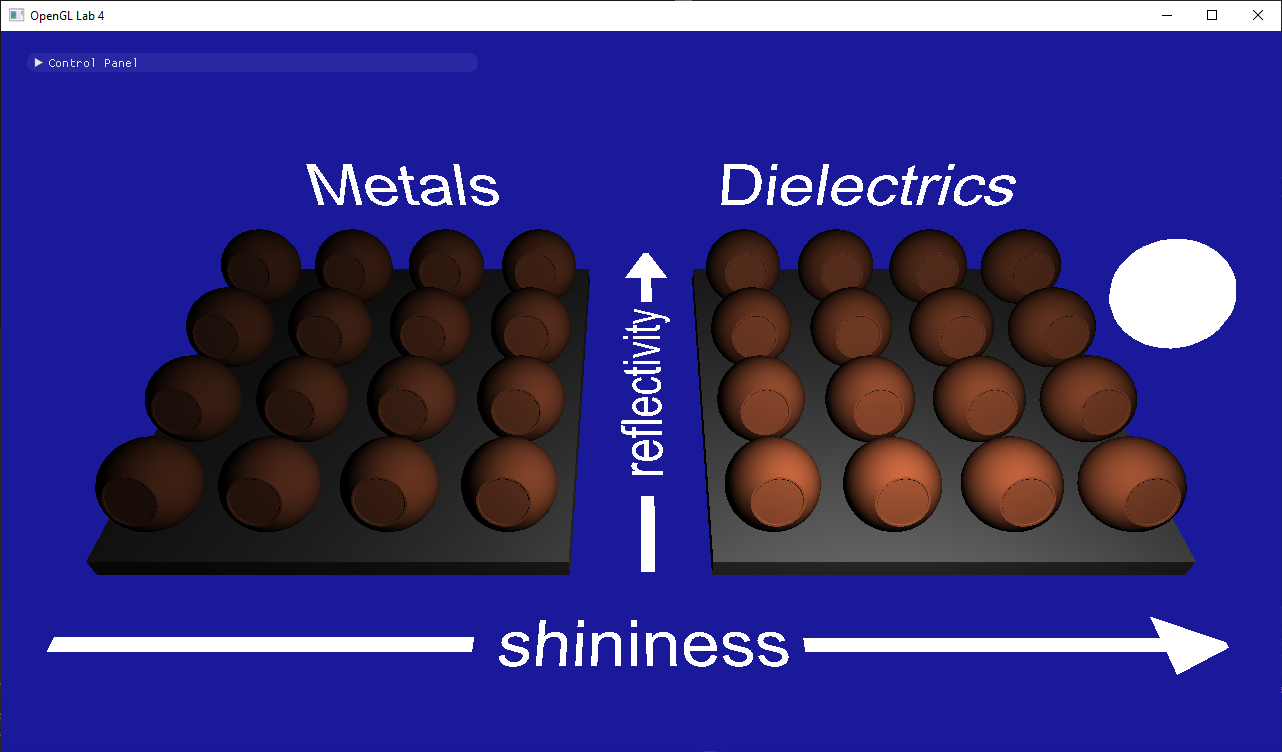
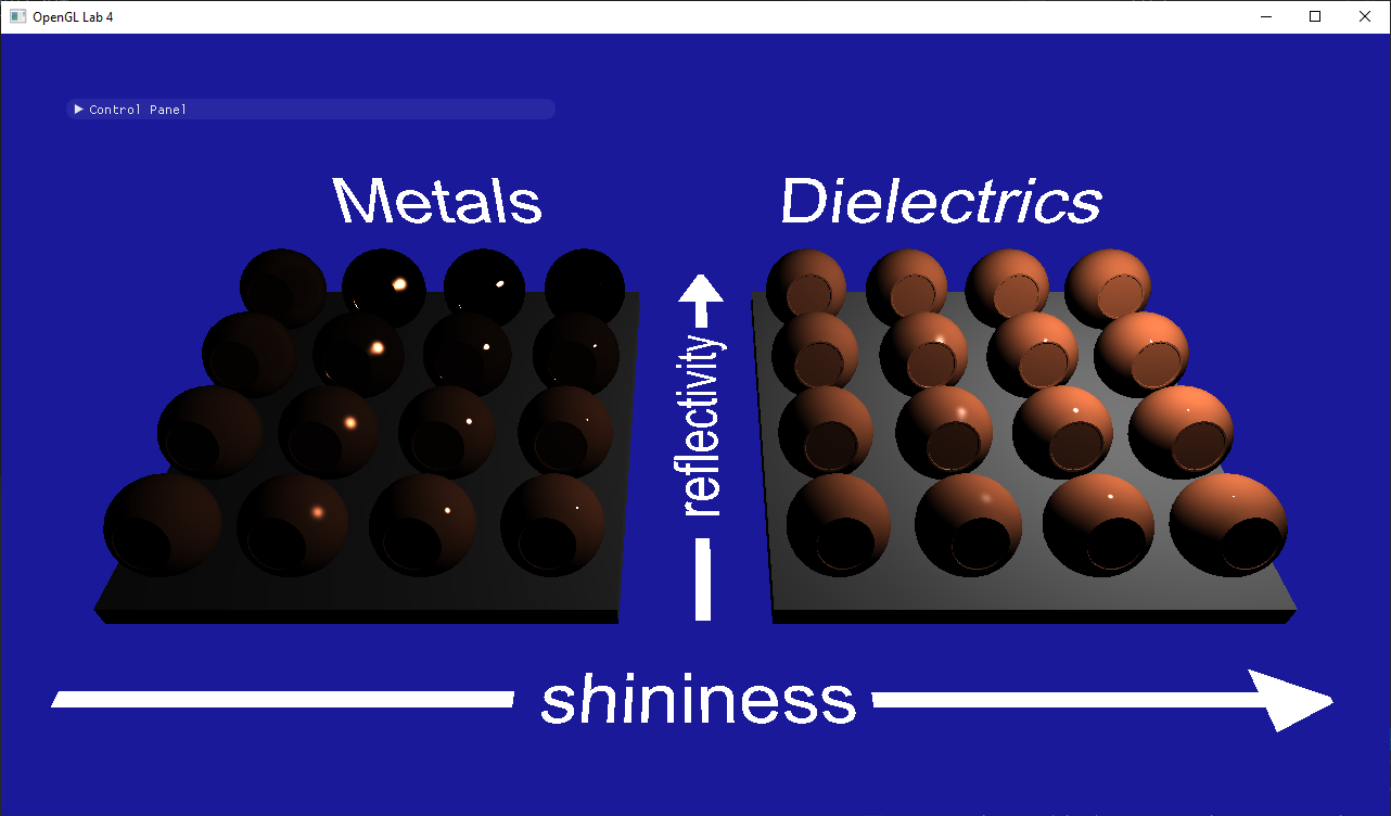
lab4_main.cpp, find where the NewShip.obj model is chosen, and choose the materialtest.obj scene instead. Run the program again:

// MaterialTest ///////////////////////////////////////////////////////////////
vec3 cameraPosition(0.0f, 30.0f, 30.0f);
vec3 cameraDirection = normalize(vec3(0.0f) - cameraPosition);
vec3 worldUp(0.0f, 1.0f, 0.0f);
const std::string model_filename = "../scenes/materialtest.obj";
///////////////////////////////////////////////////////////////////////////////

// NewShip ////////////////////////////////////////////////////////////////////
//vec3 cameraPosition(-30.0f, 10.0f, 30.0f);
//vec3 cameraDirection = normalize(vec3(0.0f) - cameraPosition);
//vec3 worldUp(0.0f, 1.0f, 0.0f);
//const std::string model_filename = "../scenes/NewShip.obj";
///////////////////////////////////////////////////////////////////////////////
Task 1

This scene has been set up so that each ball is either metal or dielectric (with suitable fresnel values) and with varying shininess and reflectivity. You can switch between scenes as you want, but this scene can be useful to verify that you are on the right track. Right now, all the balls are plain old diffuse of course. Let's fix that.

Microfacet BRDF

We are going to implement a Torrance-Sparrow Microfacet BRDF, with a Blinn-Phong Microfacet Distribution. Or, in other words, we're gonna do a shiny thing! The brdf we will implement looks like this:

brdf = $ \frac{F(\omega_i) D(\omega_h) G(\omega_i, \omega_o)}{4(n \cdot \omega_o)(n \cdot \omega_i)} $

F, the fresnel term. This term decides what amount of incoming light is going to be reflected instead of refracted. Typically, more light reflects when the incoming direction is near grazing angles. The "real" fresnel equations are rather gritty, so we will use a simple approximation (Schlick, 1994) that usually works well enough for computer graphics:

$ F(\omega_i) = R_0 + (1 - R_0) (1 - \omega_h \cdot \omega_i)^5$,

where $R_0$ (the material_fresnel uniform in your shader) is the amount of reflection when looking straight at a surface.

Task 1
Only the microfacets whose normal is $\omega_h$ will reflect in direction $\omega_o$. $D(\omega_h)$ gives us the density of such facets.
D, the Microfacet Distribution Function. This is a function that tells us the density of microfacets with a particular normal. Since all the microfacets are perfect little mirrors, only the ones that have a normal equal to $\omega_h$, the half-angle between the incoming and outgoing directions, will reflect light in the outgoing direction. We will use the normalized Blinn-Phong function discussed in the lectures:

$\omega_h = $ normalize($\omega_i + \omega_o$)
$s = $ material_shininess
$ D(\omega_h) = \frac{(s + 2)}{2\pi} (n \cdot \omega_h)^s$

Task 1
When $\omega_o$ or $\omega_i$ are at grazing angles, radiance might be blocked by other microfacets. This is what $G(\omega_i,\omega_o)$ models.
G, the shadowing/masking function. This function models the fact that if the view or light directions are close to grazing angles, the incoming or outgoing light might be blocked by other little microfacets. We will use the following function:

$G(\omega_i, \omega_o) = $ min(1, min($2\frac{(n \cdot \omega_h)(n \cdot \omega_o)}{\omega_o \cdot \omega_h}, 2\frac{(n \cdot \omega_h)(n \cdot \omega_i)}{\omega_o \cdot \omega_h}$))

Now take a deep breath and implement the brdf. Once you are done, take a look at what your surfaces would look like if they were all specular by calculating the reflected light using only this brdf and returning it:
return brdf * dot(n, wi) * Li; 
Task 1
If your image does not look almost exactly like this, it's debugging time. First of all, take a look at the image above. Does it make sense? Discuss the following with your lab-partner:
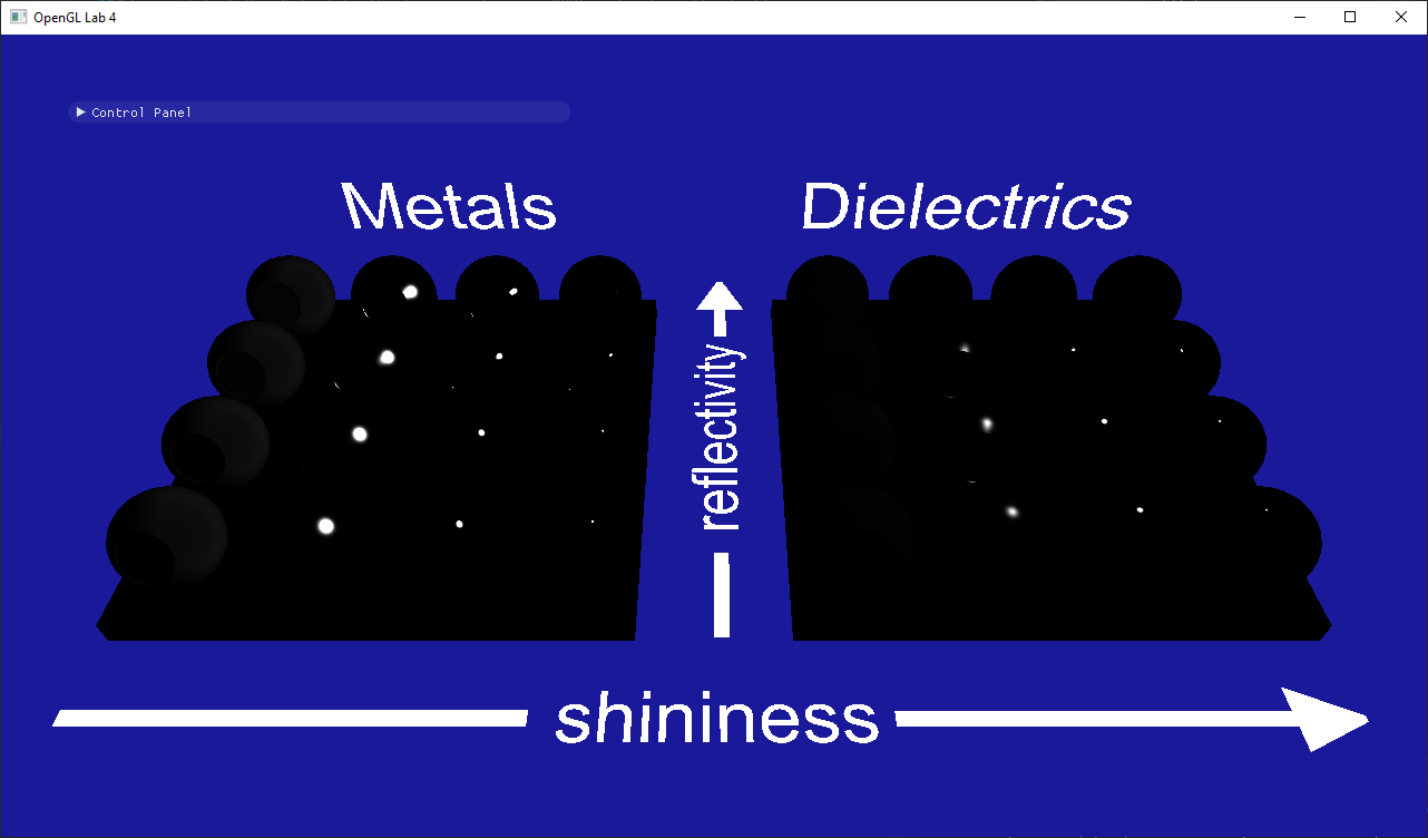
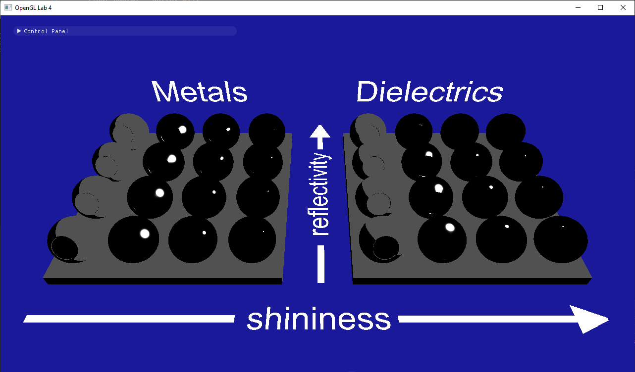
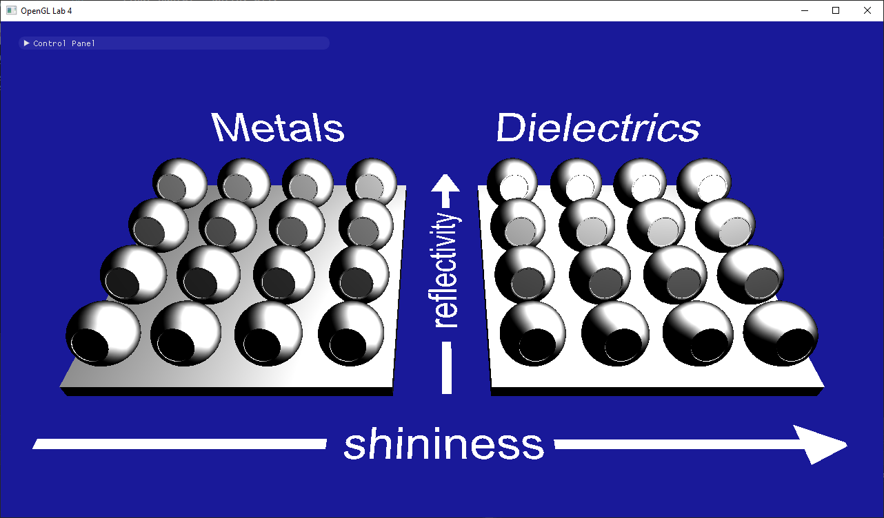
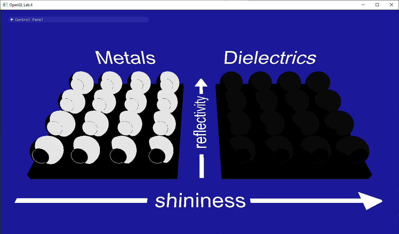
  • Why are there no colors?
  • Why are the metals with shininess 0 grayish while the dielectrics are black?

Now validate the terms one by one to find your (potential) bugs. Set lightManualOnly=true in lab4_main.cpp to get the light stopped in the right place from start.
vec3(D)
vec3(G)
vec3(F)
IF YOU GET PINK PIXELS: the last lines of code in the fragment shader are used to give a way to visually verify if there might be some problem in the implementation of these formulas. They check if the output color has a NaN (not-a-number) value and if so they paint it pink instead.
We do this because, in later labs, having single pixels with NaN value will spread around the image when we apply post-processing effects. NaN outputs should be fixed so they don't appear.
The most common operations that can result in NaNs are:
  • Division 0/0. Also
  • Multiplying 0*∞. This is basically the same problem as before, as 1/0 = ∞. Basically, try to avoid dividing by 0 (or numbers very close to it).
  • Trying to normalize a null or very short vector. Normalizing like that might internally become a 0/0 problem.
  • Square root of negative numbers. Since we are only dealing with real numbers we don't get to play with imaginary ones.
  • Power of negative numbers to exponents that are in the range $(-1, 1)$. Exponentiating to a number smaller than 1 is the same as taking some root of the number, so it's the same case as before. For example, $x^{0.5} = \sqrt{x}$.
  • acos() or asin() of values outside the $[-1, 1]$ range.

Material parameters

Good job! Now we have done all the hard stuff (in this part) and are just going to get the rest of our material system working. Let's start with the metalness parameter. If the material is a dielectric (i.e., not a metal), all the light that was not reflected should be refracted into the material, bounce around and fly out again in a random direction. We model this by letting the refracted light reflect diffusely:

dielectric_term = brdf * $(n\cdot \omega_i) L_i$ + $(1-F(\omega_i))$ * diffuse_term

If the material is a metal, all the light that was refracted will be absorbed and turned into heat. However, for a metal, we want the reflected light to take on the color of the material:

metal_term = brdf * material_color * $(n\cdot \omega_i) L_i$

Now we want to blend between these two ways of reflecting light with the $m = $ material_metalness parameter:

microfacet_term = $m$ * metal_term + $(1-m)$ * dielectric_term

Finally, we want to be able to blend between a perfectly diffuse and a microfacet brdf with the $r = $ material_reflectivity parameter:

return $r$ * microfacet_term + $(1-r)$ * diffuse_term

Great! You are done with the direct illumination. Take a breather and play around with the material properties until your spaceship looks just the way you always wanted it. The material test scene should now look like this:

Task 3

Part 2: Indirect illumination

Now stop playing, and let's get some indirect illumination going. While the first part of this tutorial was an exercise in doing everything as physically correct as we could, this part is going to contain some heavy-duty cheating. You may have noted that your scenes looks pretty dark, since they are only lit by a single point-light source. In this part we are going to add an environment map to the scene and then use that to illuminate our model.

Loading and viewing the environment map

First of all we are going to implement a helper function to render a quad (two triangles) that cover the full screen. This will only be used once now, but it will be very helpful in subsequent labs.

Look for initFullScreenQuad in lab4_main.cpp. Here you need to create the vertex array object with the geometry that will be sent to the gpu when we render a full screen quad later. Since we are always rendering the full screen we don't want to apply any projection or view matrix to these two triangles, so we can send screen space positions to the gpu directly, that way the vertex shader only has to pass them through (you can see that if you look at background.vert). The screen coordinates go from $(-1, -1)$ (bottom left) to $(1, 1)$ (top right).

Hint: In the code from lab 1 and 2 more than the position is sent to the shader. Here you should only send the positions, no normals or colors.

Also take into account that the vertex shader expects a 2 components per vertex, instead of 3 components as we sent in in previous labs.

Now go to drawFullScreenQuad, also in lab4_main.cpp, and implement here the code to draw the vertex array object you just created.

Note: you need to disable depth testing before drawing, and restore it's previous state when you are done. You can use glDisable(GL_DEPT_TEST) and glGetBooleanv(GL_DEPTH_TEST, &depth_test_enabled) to accomplish that.

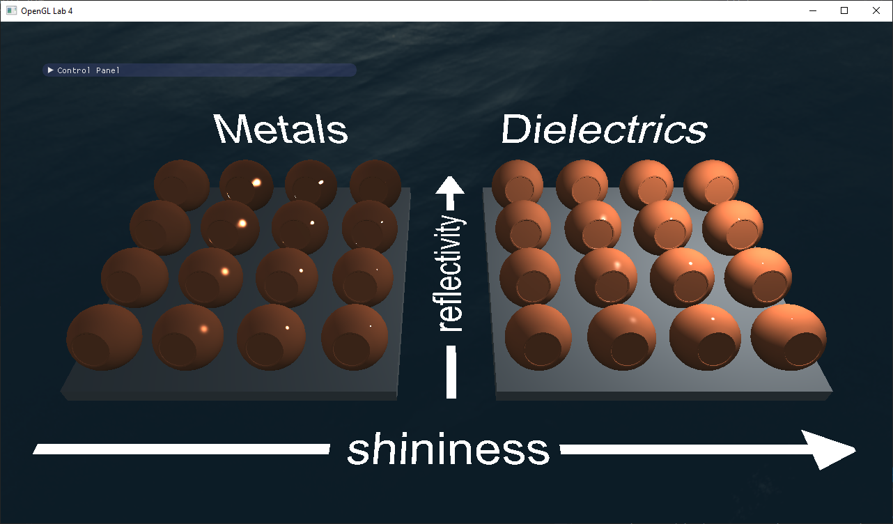
After this, we're actually already loading the environment map for you, along with some preconvolved irradiance and reflection maps (more on that later). All you have to do to see it is to add the following lines after Task 4.3 in lab4_main.cpp.

glUseProgram(backgroundProgram);				
labhelper::setUniformSlow(backgroundProgram, "environment_multiplier", environment_multiplier);
labhelper::setUniformSlow(backgroundProgram, "inv_PV", inverse(projectionMatrix * viewMatrix));
labhelper::setUniformSlow(backgroundProgram, "camera_pos", cameraPosition);
drawFullScreenQuad();

You're surrounded by water. Have a look at the environment map below. This is a sphere of incoming radiance projected onto a 2D image using the spherical coordinates. Now look at the background program shaders. All we do is render a quad that covers the whole window. Then, in the fragment shader, we figure out the world-space position of each fragment (on the near plane). We calculate the direction (still in world space) from the camera to that position, and use that direction to do a lookup in the environment map.

Task 1
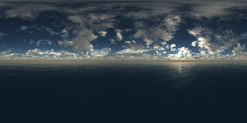
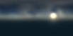
scenes/envmaps/001.hdr

Diffuse lighting with the irradiance map

Now we want to use this map to illuminate our spaceship. That is harder than it sounds. To calculate the reflected radiance that is due to indirect lighting in the direction $\omega_o$, we need to solve:

$L_o(\omega_o) = \int_{\Omega}{f(\omega_i, \omega_o)(n \cdot \omega_i)L_i(\omega_i)d\omega_i}$,

where $f$ is the brdf. This is the "Rendering Equation" that will be explained later in the course. Without going into details, it basically says that we have to look at all possible incoming directions and sum up the reflected light from that direction. One problem is that we don't have any way of obtaining $L_i(\omega_i)$ (the incoming radiance from any of the infinite directions $\omega_i$). To do that, we would have to do some kind of raytracing. That's an easy way to get pretty far from the realtime speeds we are trying for. We do have our environment map though, so if we completely ignore the fact that some of the rays we shot would be blocked by geometry, we could just use the radiance we can fetch in the environment map!

However, to estimate this integral, we would still have to take many many samples from the environment map for every single fragment. Let's start by looking at the easier problem of solving this only for diffuse reflections. At diffuse surfaces, the brdf is constant:

$L_o(\omega_o) = \int_{\Omega}{\frac{1}{\pi} c (n \cdot \omega_i)L_i(\omega_i)d\omega_i} = \frac{1}{\pi} c \int_{\Omega}{(n \cdot \omega_i)L_i(\omega_i)d\omega_i}$

Now the integral is an expression that only depends on $n$! So, we can precompute this for every possible $n$ and store the result in a 2D image just like our environment map. Fortunately, we have already done that for you, and saved the result as 
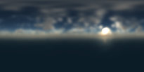
scenes/envmaps/001_irradiance.hdr. Look at the contents of that image (below) and make sure you understand what it contains. We also load it and send it to the shader so all you have to do is the lookup.

Task 1
scenes/envmaps/001_irradience.hdr

Actually, you will also need the world-space normal to do the lookup, but you can get that by simply transforming the view-space normal with the inverse of the view-space matrix, which is sent to the shader. In the calculateIndirectIllumination() function, steal the code from the background shader that calculates the spherical coordinates of a direction to fetch radiance, and use it to fetch the irradiance you want from the irradiance map using the world-space normal $n_{ws} = $ viewInverse * $n$.

Then use this to calculate your diffuse_term = material_color * (1.0 / PI) * irradiance and return that value. Now run you code and enjoy the result:

Start State

Note that the resulting reflections are rather subtle. If you want to make sure you got it right, turn your light intensity down to zero. Your balls are now only lit by the irradiance map. Make sure the are brighter on the side that faces the sun and pretty dark on the bottom.

Glossy reflections using preconvolved environment maps

Now we're getting somewhere! But we would still like to get those nice microfacet reflections from the environment as well. This is where we have to really start cheating. We can't properly precompute the result, as we did for the diffuse reflections, because the precomputed result would depend on both the normal and the incoming direction, so we would need a 4D texture, and that is too expensive. What we will do, and what many games do, is to preconvolve the environment map with the Phong lobe, and then, whatever roughness our material really has we will treat it as though it was a perfect specular surface, and hope that it looks allright.

We have done the first step for you. The environment map has been preconvolved (think "blurred") eight times, for eight different roughnesses. These eight images are stored in the same texture as different levels of a mip-map hierarchy. Take a look at the images in the scenes/envmaps/ folder (or the first four below) to see what we have done.

Task 1 Task 1 Task 1 Task 1 scenes/envmaps/001_dl_[0-4].hdr

So, first you need to calculate the reflection vector, $\omega_i$, and transform that to world-space (Hint: Take a look at the glsl reflect() function). Then calculate the spherical coordinates (Hint: Look in the background.frag shader) and look up the pre-convolved incoming radiance using:

roughness = $\sqrt{\sqrt{2 / (s + 2)}}$
$L_i$ = environment_multiplier * textureLod(reflectionMap, lookup, roughness * 7.0).xyz

Here, $s$ is the shininess of the material, and we do the conversion to roughness because we need a parameter that varies linearly to choose a mipmap hierarchy.

Now that we have our incoming radiance, we calculate:

dielectric_term = $F(\omega_i) L_i$ + $(1-F(\omega_i))$ * diffuse_term
metal_term = $F(\omega_i)$ * material_color * $L_i$

Then calculate your final return value using material_metalness and material_reflectivity just as you did for the direct illumination. Now start the program again and pat yourself on the shoulder.

Start State
Start State

When done, show your result to one of the assistants. Have the finished program running and be prepared to explain what you have done.