This is an old website! For the current version, visit: http://www.cse.chalmers.se/edu/course/TIN172/
Here are suggested solutions to some of the example examination questions.
In the following answer for the SimCity game, I have answered from the viewpoint of the system. For the player of the game, some things (e.g., observability) would be different.
Take these answers with a grain of salt in this specific case, you could almost answer anything if you have a good explanation and depending on how you imagine the game. The question is more straightforward for a game such as chess.
| Dimension | Possible values | Value(s) | Explanation |
|---|---|---|---|
| Modularity | (F)lat / (M)odular / (H)ierarchical | M or H | Depending on how complex you imagine the game, but certainly not (F)lat |
| Representation | (S)tates / (F)eatures / (I)individuals+relations | I | The city contains simulations of persons and objects, and relations between them |
| Planning horizon | (S)tatic / (F)inite / (I)ndefinite / i(N)finite | N | There is no explicit ending goal in this game, it can continue forever |
| Observability | (F)ull / (P)partial | F | The system knows everything about everything that happens in the world |
| Dynamics | (D)eterministic / (S)tochastic | S | In the real world, things happen by chance, and they should do so in a simulation too |
| Preference | achievement (G)oals / (C)omplex preferences | C | The system does not try to “win” or “succeed” |
| Number of agents | (S)ingle / (M)ultiple | S or M | (S)ingle in the sense that there is one player, but (M)ultiple if one views the simluated persons as agents themselves |
| Learning | knowledge is (G)iven / learned from (D)ata / learned from (E)xperience | E | A good simulation engine adapts its behaviour after the player |
| Computational limits | (P)erfect rationality / (B)ounded rationality | B | An interesting city simulation contains too many possible states and actions, so the system cannot do a full search |
(a) The size is 4 × M × N, since the car can be in any of the M × N cells, and can be facing in any out of 4 directions. e from the start state.
(b) The car can turn left and right, and (sometimes) move forward. So the maximum branching factor is 3.
(c) Manhattan distance is not admissible, because of the outer wall openings. (But it is possible to modify the distance to “wrap around” horizontally, to make it admissible.)
See the animation.
For lowest-cost search (also called uniform-cost search), see http://en.wikipedia.org/wiki/Uniform-cost_search#Example.
Left to the reader.
(a) First we calculate the total cost to get to each node, by taking the difference between the numbers in each pair:
Then we get the edge costs by subtracting the node costs from each other:
We cannot deduce the cost of the DE edge, since the total path cost to E via D (which will be at least 5) will anyway be higher than the best cost to E (which is 3).
(b) It’s not admissible. The edge heuristics at node C says that the remaining path length is 2, but the real remaining length is 1.
(a) There are 3 variable nodes, A, B and C, and 3 constraint nodes which are connected to variables like this:
(b) First we can apply the (<) contraints a number of times to get the following domains:
Then we can apply the sum constraint and see that A=3 is impossible (since 3+2+3>7), B=4 is impossible (since 1+4+3>7), and that C=5 is impossible (since 1+2+5>7). Then AC is finished.
| Variable | Values before AC | Values after AC |
|---|---|---|
| A | {1,2,3,4,5} | {1,2} |
| B | {1,2,3,4,5} | {2,3} |
| C | {1,2,3,4,5} | {3,4} |
Note that there is only one solution to the problem (A=1, B=2, C=4), but AC cannot draw that conclusion. E.g., B=3 cannot be removed by AC for any of the constraints:
Left to the reader
(a) We can use 5 variables, one for each class (c1,c2,c3,c4,c5). Their domains are {A,B,C}. The constraints say that one professor cannot be in two overlapping classes:
(b) Left to the reader
(c) Left to the reader
Left to the reader
Left to the reader
(a) The BU procedure is nondeterminstic, so here is one possible run:
(b) Left to the reader
(c) Here is one possible derivation:
(a) There are lots of them, but here are two:
(b) Examples:
(c) b, c, d, f
(d) a, e, g, h
Independence means that P(X,Y) = P(X)P(Y), so the table gives us:
The rest is simple math.
Look at Piazza.
(a) The probability table is this:
| Cab | P(Cab) | Witness | P(Witness | Cab) |
|---|---|---|---|
| blue | 0.15 | blue | 0.80 |
| green | 0.20 | ||
| green | 0.85 | blue | 0.20 |
| green | 0.80 |
Bayes rule gives us:
The denominator can be calculated by summing the disjoint possibilities:
All needed probabilities can now be read off the table:
(b) Left to the reader
(a) The initial factors are:
(b) We start with the initial factors f0…f4, and eliminate variables one at the time, creating new factors:
Now only f0(C) and f8(C) are left, so we create a final factor f9(C) = f0(C) × f8(C). The probability can be calculated thus:
P(C | ¬A) = f9(C) / ΣC f9(C)
Left to the reader
Left to the reader
See Piazza.
The decision network is like the belief network in figure 6.22 (exercise 6.8), with the following additional nodes and edges:
There is one additional table representing the utility function:
| Core overheat | Shut down | Utility |
|---|---|---|
| yes | yes | − cs |
| yes | no | − cm |
| no | yes | − cs |
| no | no | 0 |
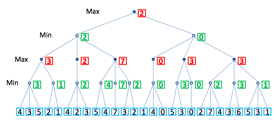
(a) Here are all min/max values at the nodes in the tree:
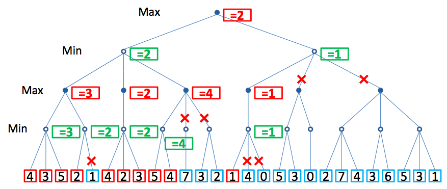
(b) Here are all min/max values at the nodes in the tree, and the αβ pruned edges:
Clarification: Some of you have noted that there is a discrepancy between the min/max values in this tree, and what is returned by the algorithm in the course book. E.g.:
For the green MIN node that is labeled “=4” (the one with children 5, 4), the book algorithm will return 2, since that is its β value.
The same for the red MAX node that is labeled “=1” and the green MIN node above. The book algorithm returns α = 2 for the MAX node and β = 2 for the MIN node.
This is not important for the final result of the algorithm – all variants of αβ pruning gives the same result in the end, and they will prune exactly the same edges. In an exam you will get correct regardless if you write the pruned MIN/MAX value (as in the tree above), or the returned α/β value (as in the book algorithm).
These are left to the reader