Lab 4: Calculator
In this lab you are going to define the main parts of a program for visualising simple functions. Running your completed lab should result in a web page looking something like this:
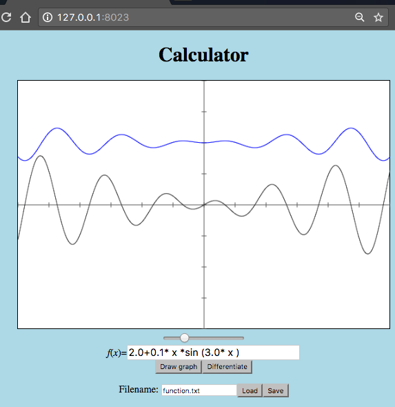
Finished Lab
The page consists of a drawing area and a text entry field below it. The user can type mathematical expressions in the text box, which, after pressing the Draw graph button, will be graphically displayed on the drawing area. The graph of the function is drawn in blue, and its first derivative in grey. You can also save/load an expression from/to a file.
The assignment
You will not need to write all the Haskell code needed to implement the calculator yourself: as usual we provide some modules that help with the user interface, and you write the interesting parts that parse expressions, calculate their derivative, read and write them, and construct the graph to be displayed in the form of an abstract picture (using a data type Picture similar to the one you used in Lab 1).
As usual follow the standard submission instructions.
Deadlines
The lab consists (again) of two parts. Part I of the lab needs to be submitted before Monday, October 9 at 12:00 (2017).
Part II of the lab needs to be submitted before Monday, October 16 at 12:00 (2017).
There are also possible extensions suggested for the more ambitious. You can choose freely whether you want to implement these.
The final deadline for passing the lab is on Wednesday, November 1 at 23:59.
Preparations
The lab builds on material from weeks 5 and 6 – namely modelling and parsing arithmetic expressions.
Before you start working:
For the graphical user interface (GUI) we are going to use a library called ThreePennyGUI – a simple library that uses your web browser to display the user interface. To install this library type the following command in a terminal window:
cabal install threepenny-guiDownload and unzip the file
Calculator.zip. This will give you the following Haskell modules:ThreepennyPictures.hs, which provides typesPictureandColour, and the following functionsblank :: Picture (&) :: Picture -> Picture -> Picture pictures :: [Picture] -> Picture path :: [Point] -> Picture coloured :: Colour -> Picture -> Picture black,white,red,green,blue,cyan,magenta,yellow,orange :: Colour grey :: Double -> Colourwhere
type Point = (Double,Double), and the functionpathcreates aPictureconnecting a list of points together.ThreepennyGUI.hswhich providesrunCalculatorwhich will be used in yourmainfunction.ThreepennyPages.hsa helper library which is only used internally byThreepennyGUI.hs(and which you do not need to understand at all).Calculator.hswhich is the skeleton file where you will do all your programming in this lab.
Before starting on this lab, make sure that you have understood the material from the lectures on recursive data types in week 5 (part A) and week 6 (for part B). Note that a large part of this lab is mainly about modifying and extending the data type and functions from these lectures. That is, you are not supposed to invent new methods here. Rather, the point is to be able to read and understand the lecture material well enough to do some useful extensions/adjustments to it.
Good luck!
Part A: Expressions: Evaluate, Derive and Draw
In this part, you are going to design a datatype for modelling mathematical expressions containing a variable x. For example: 3*x + 17.3 * sin x + cos x * sin (2*x + 3.2) + 3*x + 5.7 In other words, an expression consists of:
- Numbers; these can be (positive) integers as well as floating point numbers
- Variables; there is only one variable,
x - Operators; for now it is enough with
+and* - Standard functions; this is a fixed set, so for now it is enough with
sinandcos
You will also implement a number of useful functions over this datatype. Put the answers to all the lab in a module called Calculator.hs where we have provided a few types and definitions.
- A01
- Design a recursive datatype
Exprthat represents expressions of the above kind. You may represent integer numbers by floating point numbers; it is not necessary to have two different constructor functions for this.
You should not just copy the datatype from the lectures, but use just one constructor in the data type Expr for each kind of expression listed above. In the lectures for example, we had one constructor Add :: Expr -> Expr -> Expr and one Mul :: Expr -> Expr -> Expr. This led to a lot of cut-and-paste code. You should avoid this here. Feel free to add your own helper data types if you find this useful.
Hints: think carefully about how you want to represent the variable x. There is a difference between the Expr data type from lecture 5B part 2: in your data type you only have to represent one variable, called x, whereas in the lectures we allowed for several different variables!
- A02
Implement function
that converts any expression to string. Use as few parentheses asshowExpr :: Expr -> String
possible. The strings that are produced, when displayed usingputStr, should look something like the
example expressions and function definitions shown earlier.
It is not required to show floating point numbers that represent integer numbers without the decimal part. For example, you may choose to always
show 2.0 as “2.0” and not as “2”. (But you are free to handle integer
numbers if you want.)
Parentheses are required only in the following cases:
- When the arguments of a
*-expression use+. For example:(3.1+4.2)*7 - When the argument of
sinorcosuses*or+. For example:sin (3.2*x) - In all other cases, you should not require parentheses. For example:
- Allow
2*3+4*5instead of2*3+(4*5) - Allow
sin xinstead ofsin(x) - Allow
sin cos xinstead ofsin (cos x)(this is different from Haskell!) - Allow
sin x + cos xinstead of(sin x) + (cos x)
- Allow
It might be a good idea to list these examples in a definition and use them as test cases for various functions.
If you want to, you can from now on use this function as the default
show function by making Expr an instance of the class Show:
instance Show Expr where show = showExprBut you do not have to do this. (Also: see the hint on testing below!)
- A03
Implement a function
that, given an expression, and the value for the variableeval :: Expr -> Double -> Doublex, calculates
the value of the expression.- A04
Implement a function
to calculate the derivative of an expression (with respect toderive :: Expr -> Exprx). Note that for the derivation of sin and cos you need to use the chain rule.- A05
You now have enough pieces to draw the graph of a given expression. In this part question you are to implement a function
wheredrawGraph :: (Double,Double) -> Double -> Expr -> PicturedrawGraph (width,height) scale exprwill create the picture that will be displayed by the GUI. (Before you try to run the program, read the information below).
We have provided a dummy definition of drawGraph which just draws a red square. To see this in action, type main in ghci and open the web page as suggested. See what happens when you move the slider.
This function will be responsible for producing everything which is visible inside the white drawing area. Your task is to create a Picture containing
- the graph of the expression,
- its derivative (drawn in a different colour), and
- (Optional, but a good exercise) the x and y axes with the scale marked as in the screenshot above.
The first argument (width,height) of drawGraph is the size of the drawing area (called the canvas) measured in pixels (the smallest unit of a digital image). (The drawing area in the GUI of this lab is 600 x 600 pixels, but that does not matter here as your function should work for any positive size). Note that the coordinate (0,0) is the center of the drawing area, just like in code.world. To draw the graph of an expression there should be one point in the graph drawn for each pixel on the x-axis (and these points are joined together into a picture using the path function). You do not need to worry about the y coordinate being outside the canvas as the GUI will just ignore those points.
The second argument scale will be the scaling factor for the image - it controls how much we zoom in when displaying the image. The scaling value tells you the ratio between pixels and floating point numbers. For example, if the scale is 2 then we are zooming in by a factor of 2. Thus point (1,1) on the canvas represents the point (2,2). But that also means that when we draw the points of the graph of an expression, we will need one point for x value 0.5 (which will be drawn at x-coordinate 1 on the canvas).
Hints: It is probably a good idea to define the following two local helper functions:
 where
   pixToReal :: Double -> Double
   -– converts a pixel x-coordinate to a real x-coordinate
   pixToReal x = ...

   realToPix :: Double -> Double
   -– converts a real y-coordinate to a pixel y-coordinate
   realToPix y = ...
To get the GUI to use your function, do the following: - create a definition sinx :: Expr defined as your representation of the expression sin(x) (for example). - edit the definition of readExpr (which you will define properly in Part B) so that it always returns Just sinx. When you have finished your definition of drawGraph the program should look like this:
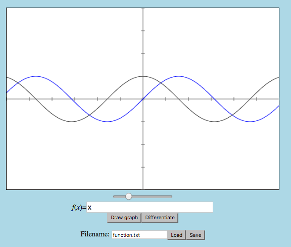
When you move the slider the image should zoom in (the slider provides scaling factors in the range [5 .. 200]).
Part B
Part B of the lab starts with the problem of Parsing, the topic covered in week 6. You should adapt the parser given in the lecture to work for your data type.
- B01
Give the proper implementation of the function
that, given a string, tries to interpret the string as an expression,readExpr :: String -> Maybe Expr
and returnsJustof that expression if it succeeds. Otherwise,Nothing
will be returned. Once this is working you can play with it in the GUI program: type in an expression and it should be displayed in the canvas area. Whenever this function returnsNothingthe GUI will warn of “syntax error”.
Hints: - Compared to the parser from the lecture, to be able to parse floating point numbers (Doubles) and sin and cos, you only have to change the parser for factors. - To parse floating point numbers, do not try to use the function “number” from the lecture, instead take a look at the standard Haskell functions read and reads. Use it on the right type (Doubles), and see what happens!
      Main> read "17.34" :: Double
      ...
      Main> read "17.34cykel" :: Double
      ...
      Main> reads "17.34cykel" :: [(Double,String)]
      ...
Before you begin the next assignment, try out your function on all the examples given in question A02 and check that they give the right expression. If you have a hard time understanding the generated counter examples for your property, it is probably a good idea to let Haskell derive the show function for your Expr datatype, instead of making your own instance of Show. So, use “deriving Show” on your expression datatype while testing!
The next assignment is about testing that your definition of readExpr matches up with your definition of showExpr.
One could define a property that simply checks that, for any expression e1, if you show it, and then read it back in again as an expression e2, then e1 and e2 should be the same.
However, this is too strict; there is certain information loss in showing an expression. For example, the expressions “(1+2)+3” and “1+(2+3)” have different representations in your datatype (and are not equal), but showing them yields “1+2+3” for both.
The lecture notes on recursive data types from week 6 gives two methods for solving this problem – one using eval and one using assoc. In this lab you should only use the assoc method. The reason for not using the eval method is that this lab uses floating point numbers, and due to rounding errors eval may give different results for the expressions x+(y+z) and (x+y)+z, and because of functions sin and cos these errors are not always small.
- B02
Write a property
prop_ShowReadExpr :: Expr -> Boolthat says that first showing and then reading an expression (using your
functions showExpr and readExpr) should produce “the same” result as the expression you started with.
Also define a size-dependent generator for expressions:Do not forget to take care of the size argument in the generator.arbExpr :: Int -> Gen Expr
Make Expr an instance of the class Arbitrary and QuickCheck the
result!- B03
The final exercise is a simple one that requires you to write a couple of small functions that allow you to save an expression to a file, and load an expression from a file. Define functions:
which save and load an expression from a file. These functions should usesaveExpr :: FilePath -> Expr -> IO () loadExpr :: FilePath -> IO ExprshowExprandreadExprrespectively, so that definitions are stored as readable strings. In the case ofloadExpryou may assume that the file exists and contains a valid expression (any errors here will be handled safely by the GUI). Make sure that you don’t accidentally overwrite any important files when testingsaveExpr!
Optional Extra Assignments
You can choose freely whether to do one or more of these. You will learn more when you do! If you decide to do any of them create a copy of your completed lab first.
- C
- Increase the expressiveness of the Expr datatype by adding more functions. Add at least -, / and tan. You have to deal with what happens when a function value is undefined! An example is the function 2/x, which is undefined in the point 0.
- D
- Instead of a single expression, generalise all functions that work with type
Exprto work with a list of expressions. These can be displayed on the canvas by showing each one in a different colour. - E
Extend the
Exprdata type to allow user-defined function names. To evaluate expressions yourevalfunction will need an extra parameter. To get a value for this parameter you can add a step inmainto read and parse definitions from a file e.g. functions.txt:
Consider how you will handle recursive definitions (or how you will forbid them).wiggleup(x) = x + sin x ; teeth(x) = sin (2 * x) + cos (3 * x) ; pi(x) = 3.1415926
Submission
Submit your solutions using the Fire system. Your submission should consist of the following file:
Calculator.hs
Only submit additional files if you did any optional extra assignments.
Before you submit your code, Clean It Up! Remember, submitting clean code is Really Important, and simply the polite thing to do. After you feel you are done, spend some time on cleaning your code; make it simpler, remove unneccessary things, etc. We will ask you to resubmit your solution if it is not clean. Clean code:
- Does not have long lines (< 78 characters), and no tab characters
- Has a consistent layout
- Has type signatures for all top-level functions
- Has good comments
- Has no junk (junk is unused code, commented code, unneccessary comments)
- Has no overly complicated function definitions
- Does not contain any repetitive code (copy-and-paste programming)
- Passes the
hlintcommand without warnings
Once you have submitted, please arrange to present your solution to one of the course assistants according to the instructions on the lab overview page.
Good luck!