Links:
Introduction
Haste is a compiler from Haskell to Javascript, which is a common language for programming interactive web pages. Normally a web page consists of an HTML document which describes the static content and maybe some Javascript code that manipulates the page and perhaps interacts with the user. In this course, we will use Haste in such a way that it will produce the whole web page for us, with the Javascript included. This has the benefit that we will not have to understand anything about HTML or Javascript. The whole web page will be described in Haskell.
Before continuing, make sure that you have installed Haste:
| Note: If, for whatever reason, you’re not able to install Haste on your own computer – don’t spend too much time on it. It’s better to spend that time on the lab assignment, and just use Haste on the Chalmers computers. |
The helper functions developed in this document are available in the module Pages.hs (which is also used by the other Haskell files linked from this document).
Hello world!
Let us begin with a simple “Hello world” example:
import Haste

main = alert "Hello world!"
Compile this program by running
hastec --output-html HelloWorld.hsThis produces a file HelloWorld.html which, when loaded in the browser, displays a simple text box.
Content and layout
The first step in making an interactive web page is to add some content, content that can later be manipulated as part of the user interaction. To do this, one has to have some understanding of the fact that a web page is represented as a tree structured object in the browser, the so-called Document Object Model (DOM).
A simple web page that just contains a single piece of text can be defined as follows:
main = do
    text <- newTextElem "This is some text."
    appendChild documentBody text
The first line in the do block creates a so-called “element” that contains the text, and the second line adds this element as a child to the document body (documentBody is the root of the visible part of the document tree).
In this course we will not be much concerned with creating textual web pages – we are more interested in graphical and interactive elements. To begin with, we need to be able to create various elements and place them according to some layout. There are different ways to create layouts, but we will just use a very simple “column-of-rows” approach.
To add a number of “child” elements in sequence to a “parent” element, we just use appendChild multiple times in sequence:
main = do
    text1 <- newTextElem "This is some text."
    text2 <- newTextElem "More text."
    appendChild documentBody text1
    appendChild documentBody text2
This produces a page displaying the text “This is some text.More text.”; i.e. the two texts have been placed in sequence. For adding a list of elements to a parent, we use the following helper function:
appendChildren :: Elem -> [Elem] -> IO ()
appendChildren parent children = sequence_ [appendChild parent c | c <- children]
If the children are “simple” elements (e.g. text elements, as above) appendChildren will place them horizontally, so we give appendChildren an alternative name to signify the fact that we can use it to construct rows in our layouts:
row :: Elem -> [Elem] -> IO ()
row = appendChildren
(Note that the Elem type represents nodes in the DOM tree.)
By using row, our example becomes slightly simpler:
main = do
    text1 <- newTextElem "This is some text."
    text2 <- newTextElem "More text."
    row documentBody [text1,text2]
Our next step is to place elements on top of each other to achieve vertical layout. This is done in almost the same way as when creating a row, except that we first need to wrap all children in a “div” element. The wrapping is done as follows:
wrapDiv :: Elem -> IO Elem
wrapDiv e = do
    d <- newElem "div"
    appendChild d e
    return d
The effect of wrapping an element in a “div” node is that it will use up the full horizontal width so that elements next to it will be placed above or below it. Note that although newElem can be used to create a new element of any name, there are only a predefined set of elements which the web browser understands. “Div” is one of them.
Now the definition of column:
column :: Elem -> [Elem] -> IO ()
column parent children = do
    cs <- sequence [wrapDiv c | c <- children]
    appendChildren parent cs
To demonstrate how to use row and column to create layouts, we give the following example that places four elements in two rows:
main = do
    text1     <- newTextElem "top left "
    text2     <- newTextElem "top right "
    text3     <- newTextElem "bottom left "
    text4     <- newTextElem "bottom right "
    topRow    <- newElem "div"  -- Container for the top row
    bottomRow <- newElem "div"  -- Container for the bottom row
    row topRow [text1,text2]
    row bottomRow [text3,text4]
column documentBody [topRow,bottomRow]Since row needs to have a parent element to add the children to, we had to create two extra elements topRow and bottomRow to contain the two rows. “Div” elements for this purpose.
Although the above example may seem very stupid as a way of laying out text, it will turn out quite useful when we consider layout of interactive and graphical elements.
Interactive web pages
To create pages that react to user input one can make use of buttons and text entries (“button” and “input” elements respectively). Here is a simple example that makes a text entry with a button below it:
main = do
    input  <- newElem "input"
    button <- newElem "button"
    set input
        [ prop "type"  =: "text"
        , prop "size"  =: "30"  -- Width of box
        , prop "value" =: "Type your answer here..."
        ]
    set button [ prop "innerHTML" =: "Submit answer" ]
    column documentBody [input,button]
This example will be displayed as follows in the browser:
The set instructions are used to set various properties of the new elements. We will not go into details of these properties here; whenever you need an input box or a button, you can just copy the above code and alter the relevant strings.
In order to make creation of input boxes and buttons easier, we define two helper functions:
mkInput :: Int -> String -> IO Elem
mkInput width init = do
    input <- newElem "input"
    set input
        [ prop "type"  =: "text"
        , prop "size"  =: show width
        , prop "value" =: init
        ]
    return input

mkButton :: String -> IO Elem
mkButton label = do
    button <- newElem "button"
    set button [ prop "innerHTML" =: label ]
    return button
Now it is time to make the page interactive! Let’s say we want the text in the box to change when the button is clicked. Here is how to do that:
main = do
    input  <- mkInput 30 "Type your answer here..."
    button <- mkButton "Submit answer"
    column documentBody [input,button]

    onEvent button Click $ \_ -> do
      set input [ prop "value" =: "You clicked!" ]
Again, we will not go into the details of how this works, but intuitively, the last part sets an “event handler” that will be called whenever the button is clicked. In this case, the event handler simply changes the text in the input element, but of course, handlers can be arbitrarily complex.
The argument to the handler (which we ignore by using _) gives information about of the click (mouse position, etc.). This is can be useful e.g. to catch mouse clicks in a game, but in this example we do not make use of it.
The following example demonstrates how to read the text in the input box and copy it to a different place in the page while the user is typing:
main = do
    input  <- mkInput 30 ""
    output <- newElem "span"
    column documentBody [input,output]

    onEvent input KeyUp $ \_ -> do
      text <- getProp input "value"
      set output [ prop "innerHTML" =: text ]
    focus input
Here we use a “span” element to hold a piece of text that is placed below the input box. An event handler made from KeyUp will run whenever a keyboard key is released, i.e. after every typed character in the input box. The event handler reads the contents (the “value” property) of the input box and copies that to the output element.
The command focus input makes the input box the currently active element, so that the user can start typing without first clicking in the box.
Calculator.hs is a similar example, but where the script actually computes a result, rather than just copying text.
Graphics in the browser
The HTML5 standard includes a “canvas” element for drawing figures in the browser. In our examples, we will use the following function to create a canvas of a given width and height:
mkCanvas :: Int -> Int -> IO Elem
mkCanvas width height = do
    canvas <- newElem "canvas"
    setStyle canvas "border" "1px solid black"
    setStyle canvas "backgroundColor" "white"
    set canvas
        [ prop "width"  =: show width
        , prop "height" =: show height
        ]
    return canvas
In order to interface with the canvas from Haskell code, one first has to import Haste’s canvas library:
import Haste.Graphics.CanvasThis library contains two types used for creating pictures: Shape and Picture. Basic shapes can be created using the basic functions
line   :: Point -> Point -> Shape ()
rect   :: Point -> Point -> Shape ()
circle :: Point -> Double -> Shape ()
A Point is a pair of floating point numbers corresponding to the number of pixels in the x and y dimension, respectively:
type Point = (Double,Double)Combining pictures
Shape is an “instruction type” just like e.g. IO, which means that we can use do notation to combine shapes:
snowMan :: Double -> Shape ()
snowMan x = do
    circle (x,100) 20
    circle (x,65) 15
    circle (x,40) 10
Once we are done with a Shape, it can be turned into a Picture in two basic ways:
fill   :: Shape () -> Picture ()
stroke :: Shape () -> Picture ()
The former function fills the shape with solid color, while the latter only draws the contours. Picture is also an “instruction” type, so pictures can be combined using do-notation:
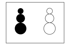
twoSnowMenInABox :: Picture ()
twoSnowMenInABox = do
    fill   $ snowMan 100
    stroke $ snowMan 200
    stroke $ rect (50,10) (250,150)
This will result in the following picture:
The main function to draw the picture is the following:
main :: IO ()
main = do
    canvas <- mkCanvas 300 300
    appendChild documentBody canvas
    Just can <- getCanvas canvas
render can twoSnowMenInABoxAnimations
It is possible to animate pictures in a canvas simply by periodically redrawing the picture. FallingBall.hs is a simple animation of a falling ball. Here, the animation is achieved by the function fall recursively calling itself after a time-out of 20 milliseconds. The y argument of fall acts as the state of the animation; by increasing y in the recursive call, a slightly different picture is drawn in each iteration.
Finally BouncingBalls.hs is a more advanced animation, where the state is updated interactively by clicking in the canvas using the mouse. For this, an IO reference is used to hold the current state.