Introduction
In this final project, you will write a path-tracer capable of rendering photorealistic images (if fed with something more photorealistic than a weird spaceship). The focus here will be on correctness, rather than speed and unlike the images you have rendered in previous labs, which are complete in a few milliseconds, you may have to wait for hours for your best work to look really good. Path tracing is one of many algorithms used for off-line rendering, e.g., when rendering movies.
Path tracing is based on the concept of "ray tracing", rather than "rasterization" which is what you have done so far, and what GPUs do so well. Ray tracing is when we intersect a ray with a virtual scene and figure out, e.g., the closest intersection point. In this tutorial, the actual ray tracing will be done using Intel's "Embree" library, and we will focus on how to generate physically plausible images.
There will be a relatively large amount of theory in this tutorial, and some scary looking maths, but please, DON'T PANIC. The idea is that you shall get a feel for how the underlying maths work, but you will not be asked to solve anything especially difficult.
The startup code
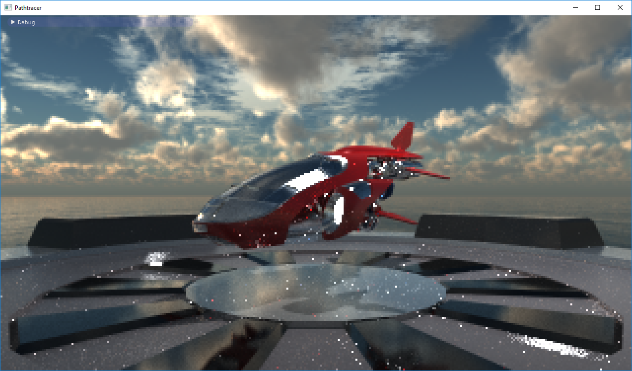
The first thing you should do (after having pulled the latest code) is to set the Pathtracer as startup project and switch to Release. Since it is highly CPU bound, this code will run extremely much slower in Debug. Both because no optimizations are turned on, and because we run on a single thread in the Debug build. So remember to run it in Release, except when you have to actually run the debugger. So, run the program. Except that it is slower, and lower resolution, you will see what should be a familiar scene by now.
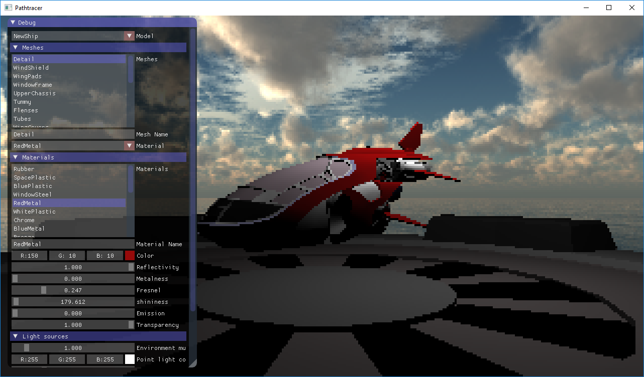
Image rendering is restarted when you move the viewpoint or change the window size, but not when you change material values in the gui.
You will recognize the GUI from Tutorial 4, but there are a few changes. You can now load several .obj models, and you can choose which you want to edit the materials for in the first drop-down list. There are also a few new settings for the path-tracer. Right now, the most important one is the subsampling setting. It simply says how many window pixels (w x h) a pixel in the raytraced image should correspond to. You may want to increase this value if you find the program to be irresponsive. The Max Bounces slider doesn't do anything yet, but you will use it later. The Max Paths Per Pixel looks like it doesn't do anything yet, but it actually says how many frames the renderer should calculate and accumulate. It will be useful later, e.g., to be able to compare images with the same quality. When it is set to zero, it will accumulate the result until you close the program (or change the view-point).
The difference is that this image is ray traced. The only thing we use OpenGL for in this program is to render a fullscreen quad, textured with the output from your raytracer. So the actual image is created on the CPU, by shooting one ray per pixel and intersecting it with the scene to find the closest intersection. For that intersection a color is calculated and accumulated to the pixel color in the rendered image.
Now let's take a look at the code, and make sure you understand how the image is generated.
main.cpp:
This should be familiar. A simple OpenGL program that draws a full-screen quad to the screen each frame and renders a GUI.pathtracer.h/cpp:
This is where the interesting stuff happens. Look attracePaths(). This code loops through all the pixels and shoots a ray for each to find an intersection point. Then theLi()function is called to calculate the incoming radiance for the intersected point. This function is where you will spend most of your efforts.embree.h/cpp:
The raytracing is handled by the external library "Embree". These files serve as an interface to that library. Have a look at the.hfile and make sure you understand what each function does. How it does it is less important for this tutorial.material.h/cpp:
These files define the BRDFs that we will use. It is pretty empty right now, but we will fill it in as we go.sampling.h/cpp:
Contain some helper functions for sampling random variables and such.
Improve the ray tracer
The
sampling.h file contains a function randf() that samples a random float $0 \leq f < 1.0$
Before we go into path tracing, let's improve this raytracer a bit.
Task #1: Jittered Sampling.
We will begin with some much needed anti-aliasing. Look at the tracePaths() function again. Every frame, we create a ray that goes through each pixel, and then we accumulate the result to the result of previous frames. Start by changing the code so that it picks a random direction within each pixel at each frame.
Task #2: Shadows
Whenever you shoot a ray, you will have to push it very slightly away from the surface you are shooting from, to avoid self intersections. Use the defined
EPSILON.
Li() function. To calculate the color of each pixel, this code does pretty much what you started with in Tutorial 4. That is, it calculates the incoming radiance from the light and multiplies this by the cosine term and the diffuse BRDF. To add shadows, you need to shoot a ray from the intersected point to the light source and find out if there is something occluding the point. Use the occluded() function, rather than intersect(). Be prepared to answer why you think we need both of these functions?
Task #3: Implement Blinn Phong BRDF
Yes, "again"! But this time you need to squeeze it into our nice little material tree. Take a look at the Li() function again. One of the first things we do is to define an object mat of the type BRDF. This is the object that we will use throughout the function to evaluate the BRDF, or sample directions. Currently, it is a simple object of type Diffuse (which inherits BRDF). Change it to be a BlinnPhong brdf, which will reflect diffusely the energy that is refracted by the Microfacet surface.
Diffuse diffuse(hit.material->m_color);
BlinnPhong dielectric(hit.material->m_shininess, hit.material->m_fresnel, &diffuse);
BRDF & mat = dielectric;As in tutorial 4 you need to make sure you don't divide by zero, and return 0 if the incoming or outgoing directions are on the wrong side of the surface.
If you run the code now, everything will be black since the BlinnPhong class is not implemented yet. Before you start doing that though, go to main.cpp and switch to only loading the simple Sphere model.
If you look at the skeleton of the class you will see that we already have some code in the BlinnPhong::f() method, but all it does is return reflection_brdf() + refraction_brdf() which both return zero. Let's change that. As in tutorial 4, the immediately reflected light should be:
$ D(\omega_h) = \frac{(s + 2)}{2\pi} (n \cdot \omega_h)^s$
$G(\omega_i, \omega_o) = $
min(1, min($2\frac{(n \cdot \omega_h)(n \cdot \omega_o)}{\omega_o \cdot \omega_h}, 2\frac{(n \cdot \omega_h)(n \cdot \omega_i)}{\omega_o \cdot \omega_h}$)) reflection_brdf() = $(F(\omega_i) D(\omega_h) G(\omega_i, \omega_o)) / (4(n \cdot \omega_o)(n \cdot \omega_i)) $
where $s$ is the material shininess and $\omega_h$ is the half-vector between $\omega_i$ and $\omega_o$.
If the light is refracted, we will hand over calculations to whatever brdf is attached as the layer below, so implement refraction_brdf() = $(1 - F(\omega_i))$ * refraction_layer->f(...) (but if it is NULL you should just return 0.)
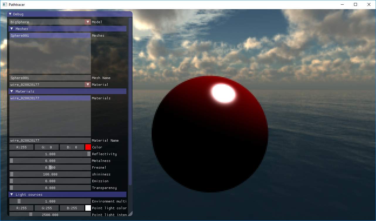
When you're done, if the sphere material is set up as below you should have something like the following result:
Task #4: Implement the material model
Now let's put the rest of the material model in place. In Li(), build a complete material like this:
Diffuse diffuse(hit.material->m_color);
BlinnPhong dielectric(hit.material->m_shininess, hit.material->m_fresnel, &diffuse);
BlinnPhongMetal metal(hit.material->m_color, hit.material->m_shininess,
                      hit.material->m_fresnel);
LinearBlend metal_blend(hit.material->m_metalness, &metal, &dielectric);
LinearBlend reflectivity_blend(hit.material->m_reflectivity, &metal_blend, &diffuse);
BRDF & mat = reflectivity_blend;LinearBlend::f(), BlinnPhongMetal::reflection_brdf(), and BlinnPhongMetal::refraction_brdf() (remember that the energy that is refracted into a metal is just absorbed and turned into heat).
When done, load the ship and landingpad again and be slightly dissapointed that everything looks a bit boring when you only do direct illumination.
Write a pathtracer
Now we are going to turn this simple ray tracer into a proper path tracer and get some proper indirect illumination into our immages. At this point there is no way to proceed without first understanding the basics of:
The Rendering Equation
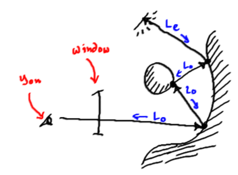
This is an formula that tells us what the outgoing radiance from some point will be, given that we know all the incoming radiance at that point. If you need more details than are given here, have a look at chapters 7 and 9 in your textbook, or cruise the internet. The equation looks like this (I have omitted the point, $p$, for brevity):
It says that the radiance (Watt per unit solid angle and unit area) $L_o$ that leaves a point in the direction $\omega$ can be found from the:
- Emitted Light: $L_e(\omega)$ - If the surface at this point emits radiance in direction $\omega$.
- BRDF: $f(\omega, \omega')$ - This is a function that describes how the surface at this point reflects light that comes from direction $\omega'$ in direction $\omega$.
- Incoming radiance: $L_i(\omega')$ - This is the incoming light from direction $\omega'$.
- Cosine term: $cos(n, \omega')$ - This will attenuate the incoming light based on the incident angle.
There is no analytical solution to this equation. We can however estimate it using what is called Monte Carlo integration, and that is exactly what a pathtracer does.
Without going into too much detail, monte carlo integration means that we can get what is called an unbiased estimator of the integral by sampling one direction $\omega'$ randomly, if we then weight our estimate by the Probability Density Function, or PDF. The PDF is (roughly) a function that tells us how likely we were to choose the random direction $\omega'$.
The fact that it is an unbiased estimator means that if we calculate:
At some intersection point, we can immediately evaluate everything in Equation 1, above, except for the $L_i(\omega_i)$ term (the incoming light from direction $\omega_i$). But the incoming radiance from some direction can be found by shooting a ray in that direction, and calculating the outgoing radiance from the first intersection point. And the outgoing radiance, we know how to estimate by looking in a single new incoming direction.
Path tracing
 What all this boils down to is the path-tracing algorithm. We start by shooting one ray per pixel (the ray starts at the camera and goes “through” the pixel and into the scene). We find the first intersection-point with the scene and there we want to estimate the outgoing radiance.
We do so by shooting one single ray to estimate the incoming radiance. At the first intersection point for that ray, we again shoot a single ray and so on, forming a path that goes on until there is no intersection (or we terminate on some other criteria). At each vertex of the path we will evaluate the emitted light, the BRDF and the cosine term to obtain the radiance leaving the point. When the recursion has terminated and we have obtained $L_o$ for the first ray shot, we record this radiance in the framebuffer.
This is all we need to do to create a mathematically sound estimation of the true global illumination image we sought! It’s probably all black though, unless we were lucky and hit an emitting surface with some rays in which case it might be black with a little bit of noise. But if we keep running the algorithm, and accumulate the incoming radiance in each pixel (and divide by the number of samples) we would eventually end up with a correct image. This will take more time than is left for this course though, so we need to speed things up a bit.
Separating Direct and Indirect Illumination The first step is to separate indirect and direct illumination. At each vertex of the path we will first shoot a shadow-ray to each of the light-sources in the scene. If there is no geometry blocking the light we will multiply the radiance from the light with the BRDF and cosine term and then add the incoming indirect light by shooting a single ray as before. For this to be correct, we just have to make sure that the surfaces we have chosen to be light-sources do not contribute emitted radiance if sampled by an indirect ray.
There! That’s a path-tracer and it generates correct images in a reasonable time.
Task #5: Implement a path tracer
So let's turn all that theory into code now. It is tempting to start writing this as a recursive function, but that will not be very efficient, and we will instead suggest an iterative approach as outlined in the pseudo code below:
L               <- (0.0, 0.0, 0.0)
pathThroughput  <- (1.0, 1.0, 1.0)
currentRay      <- primary ray
for bounces = 0 to settings.max_bounces
{
	// Get the intersection information from the ray
	Intersection hit = getIntersection(current_ray);

	// Create a Material tree
	Diffuse diffuse(hit.material->m_color);
	BRDF & mat = diffuse;

	// Direct illumination
	L += path_throughput * direct illumination from light if visible

	// Add emitted radiance from intersection
	L += path_throughput * emitted light

	// Sample an incoming direction (and the brdf and pdf for that direction)
	(wi, brdf, pdf)  <- mat.sample_wi(hit.wo, hit.shading_normal)

	cosineterm = abs(dot(wi, hit.shading_normal))

	pathThroughput = pathThroughput * (brdf * cosineterm)/pdf

	// If pathThroughput is zero there is no need to continue
	if (pathThroughput == (0,0,0)) return L

	// Create next ray on path
	currentRay <- new ray from intersection point in outgoing direction

	// Bias the ray slightly to avoid self-intersection
	currentRay.o += PT_EPSILON * isect.normal

	// Intersect the new ray and if there is no intersection just
	// add environment contribution and finish
	if(!intersect(currentRay))
		return L + path_throughput * Lenvironment(currentRay)

	// Otherwise, reiterate for the new intersection
}
Implement this in your
Li() function.
When you start testing your code, make sure you have switched back to just diffuse shading, and use the sphere model to keep things simple at first. When you are done, you should have a pathtraced image looking like this (after it has rendered for a couple of seconds): 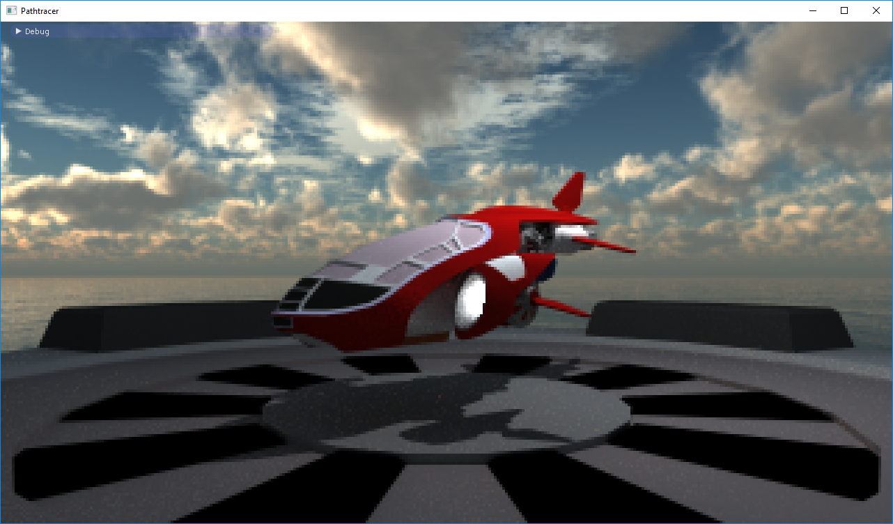
, and you can start feeling a little bit proud of yourself.
Improve the pathtracer
Let's immediately destroy that new-found self confidence. Change your material model back to a single BlinnPhong + Diffuse material again:
Diffuse diffuse(hit.material->m_color);
BlinnPhong dielectric(hit.material->m_shininess, hit.material->m_fresnel, &diffuse);
BRDF & mat = dielectric;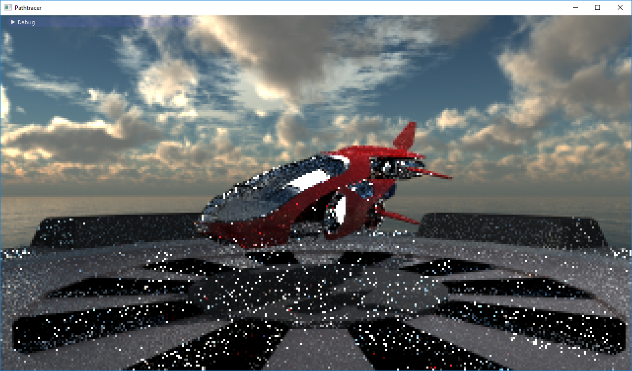
Ouch! That's not what you wanted is it? In theory, there is actually nothing wrong. If you let this image keep rendering you should eventually end up with a nice smooth image, but it could take weeks. This is because of how you choose your incoming direction, and the solution is a method called importance sampling.
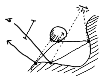
Importance Sampling
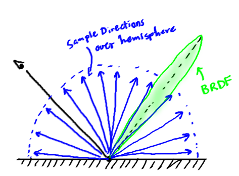
The problem is illustrated in the image to the right. Say that our BRDF represents a near mirror direction. That means that all sample directions that are not close to the perfect specular reflection direction will contribute almost nothing. But we still happily choose directions uniformly from all over the hemisphere.
With importance sampling we will instead pick samples from a distribution that looks more like the BRDF we are trying to sample, for which we know the Probability Density Function (PDF), $p(\omega_i)$.
We will now pick samples with a probability that is much higher where the BRDF is large. We then have to divide the resulting radiance of each sample by the PDF in the
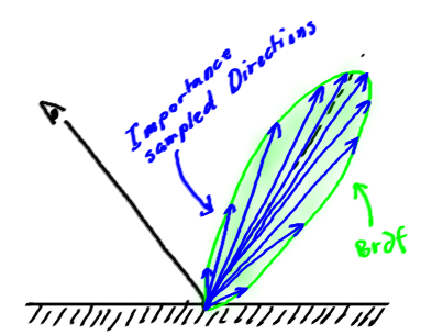 sample direction to account for this. So we will have more samples where the brdf is high, but if we happen to pick a sample where the PDF is low, its contribution will be increased.
Note that we rarely can find a sampling scheme that exactly matches the brdf and that the sampling scheme must be carefully chosen so that it will not occasionally sample directions with very low probability where the BRDF is not correspondingly low. If we do, then we can get very strong samples in some random pixels that take a very long time to converge.
Task #6: Implement importance sampling for BlinnPhong
Take a look at the current implementation of sample_wi in the BlinnPhong class. It currently chooses a direction by picking a point uniformly on a disc, and then projecting that onto the hemisphere. This gives the pdf: $p(\omega_i, \omega_o, n) = \frac{1}{\pi} |n \cdot \omega_i|$. This is great for sampling diffuse surfaces, but obviously quite poor for a mirror-like reflection.
So, in what way should we sample the incoming direction? In the best of worlds, we would have a way of choosing directions that had a pdf that was exactly proportional to our complete BRDF. But since we don't even (in this class) necessarily know what the underlying layer is, that is impossible. Instead, we will use a technique called russian roulette to randomly pick either a direction suitable for directly reflected photons or a direction suitable for whatever happens if they are refracted. We will choose one or the other with 50% probability, and then we have to boost the contribution for each by a factor of 2 (which we do by halving the pdf).
Think about this for a few seconds. We want the function to return a brdf that is: $F a + (1-F)b$. Instead, after dividing by the pdf, we are going to compute either $2Fa$ or $2(1-F)b$. Now convince yourself that if you do this infinitely many times, the sum of all of these samples is going to be correct. Then start writing your BlinnPhong::sample_wi function (pseudo code):
if(randf() < 0.5) {
	// Sample a direction based on the Microfacet brdf
	(wi, pdf) <- <...>
	pdf = pdf * 0.5;
	return reflection_brdf(wi, wo);
}
else {
	// Sample a direction for the underlying layer
	(wi, brdf, pdf) <- refraction_layer->sample_wi(...);
	pdf = pdf * 0.5;
	// We need to attenuate the refracted brdf with (1 - F)
	F <- R0 + (1.0f - R0) * pow(1.0f - abs(dot(wh, wi)), 5.0f);
	return (1 - F) * brdf;
}
Great! Now we only need to replace the <
...> with actually choosing a direction $\omega_i$ in such a way that we get more samples where the brdf is high. The actual maths for how to do this is way out of scope for this tutorial, so we will just gloss over it. It is not horribly complicated though, and we will go through it in the "advanced" course. First, we generate a half-angle vector, $\omega_h$ like this:
vec3 tangent = normalize(perpendicular(n));
vec3 bitangent = normalize(cross(tangent, n));
float phi = 2.0f * M_PI * randf();
float cos_theta = pow(randf(), 1.0f / (shininess + 1));
float sin_theta = sqrt(max(0.0f, 1.0f - cos_theta * cos_theta));
vec3 wh = normalize(sin_theta * cos(phi) * tangent +
                    sin_theta * sin(phi) * bitangent +
                    cos_theta * n);
if(dot(wo, n) <= 0.0f) return vec3(0.0f);
This vector will be chosen with a pdf: $p(\omega_h) = (s+1)(n \cdot \omega_h)^s / (2\pi)$.
But what you want is the incoming direction, $\omega_i$ which you get by reflecting $\omega_o$ around $\omega_h$. For reasons that are even more out of scope, the pdf for this vector will be $p(\omega_i) = p(\omega_h) / (4(\omega_o \cdot \omega_h))$.
Now plug in your calculations for
wi and p in your sample_wi() function and run the program again. After 1024 samples per pixel, it should look something like this:
That's much better, isn't it!? There is still noise, of course, but it mostly disappears after a few minutes or hours (depending on how fast your machine is and how may nasty little bugs are still lying around).
Task #7: Importance sample the LinearBlend.
Now we want to turn on the whole material model again. To do that we need to sample correctly for the LinearBlend brdf (the BlinnPhongMetal brdf uses the same sampling as the straight BlinnPhong already). For this BRDF, we will simply use russian roulette like before, but we will use the weight (i.e., reflectivity or metalness) to choose how likely we are to sample the one or the other underlying layers.
Project of your choice
So you say you have written a pathtracer? Grab hold of an assistant and ask him or her if they agree. When you have convinced them that your code is bug-free and everything renders exactly as it should, take a break and enjoy playing around with the materials for a while! And why not throw in a few more models and move stuff around? When you're done playing, choose one of the little projects from below and finish this off. If you have something else that you would rather add, ask an assistant if it sounds like a reasonable project.Suggested Projects
- Refraction. We have added a "transparency" property to the .obj model materials and the GUI. Change your material model so that you can make materials refractive. Have a look at Chapter 9.4 and 9.5 in the textbook for information. At a minimum you should, when finished, be able to show a glass ball that refracts its surrounding correctly (using Fresnel to calculate how much energy reflects and refracts). You get more bonus points(*) if you also calculate how energy is attenuated by transmittance. If you really want to show off, you could implement a proper rough refraction BRDF as described in, e.g., Microfacet Models for Refraction through Rough Surfaces by Walter et al.
- Area Lights. You pathtracer currently only contains one point light source. Change that, so that it contains a number of area lights instead. You should at least be able to show the assistant an image with two visible area lights (e.g. discs) that cast nice soft shadows. If you're feeling a bit ambitious you could let the light source have an arbitrary shape (by, e.g., loading an .obj model.). For extra bonus points(*) you could add Multiple Importance Sampling (google or look in any raytracing book) to improve convergence.
- Roll your own BVH. In this tutorial we have relied entirely on Intel's Embree library to do ray-tracing, but why let them have all the fun? Using the simple interface described in
embree.h replace embree with your own acceleration structure and intersection routines. Anything better than just running through a list of triangles is good enough (But an Axis Aligned Bounding Box tree is probably a good choice). Chapters 16 and 17 in the textbook should contain information to get you started. Extra bonus points(*) if you can show that your implementation is faster than Embree in any setting.
(*) Any extra bonus points are strictly ornamental. The tutorials and projects are not graded.