Hints

Some assignments have hints. Often, these involve particular standard Haskell functions that you could use. Some of these functions are defined in modules that you have to import yourself explicitly. You can use the following resources to find more information about those functions:

A Graphical Calculator

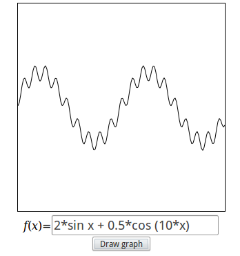
The page consists of a drawing area, and a text entry field below it. The user can type mathematical expressions in the text entry, which, after pressing the Draw graph button, will be graphically shown on the drawing area.

The lab assignment consists of two parts. In Part I, you will implement the parts of your program that have to do with expressions. In part II, you will implement the graphical part of your program.

Part I

Put the answers for Part I in a module called Expr.hs.

Assignments

A. Design a (recursive) datatype Expr that represents expressions of the above kind. You may represent integer numbers by floating point numbers; it is not necessary to have two different constructor functions for this. Your data type should be designed to make it easy to add more functions and more binary operators to the language.

B. Implement a function showExpr :: Expr -> String that converts any expression to string. Use as little parentheses as possible. The strings that are produced should look something like the example expressions shown earlier. It is not required to show floating point numbers that represent integer numbers without the decimal part. For example, you may choose to always show 2.0 as "2.0" and not as "2". (But you are allowed to do this.) If you want to, you can from now on use this function as the default show function by making Expr an instance of the class Show: instance Show Expr where show = showExpr But you do not have to do this. (Also: see the hint on testing below!)

C. Implement a function eval :: Expr -> Double -> Double that, given an expression, and the value for the variable x, calculates the value of the expression.

D. Implement a function readExpr :: String -> Maybe Expr that, given a string, tries to interpret the string as an expression, and returns Just of that expression if it succeeds. Otherwise, Nothing will be returned. You are required to use an unmodified version of the module Parsing.hs to construct this function. See the lectures from Week 4 on parsing expressions andWeek 5 on monadic parsing.

The next assignment is about checking that your definition of readExpr matches up with your definition of showExpr. One could define a property that simply checks that, for any expression e1, if you show it, and then read it back in again as an expression e2, then e1 and e2 should be the same.

However, this is too strict; there is certain information loss in showing an expression. For example, the expressions "(1+2)+3" and "1+(2+3)" have different representations in your datatype (and are not equal), but showing them yields "1+2+3" for both. The lecture from Week 4 discussed solutions to this problem.

E. Write a property prop_ShowReadExpr :: Expr -> Bool that says that first showing and then reading an expression (using your functions showExpr and readExpr) should produce "the same" result as the expression you started with. Also define a generator for expressions: arbExpr :: Int -> Gen Expr Do not forget to take care of the size argument in the generator. Make Expr an instance of the class Arbitrary and QuickCheck the result! instance Arbitrary Expr where arbitrary = sized arbExpr

F. Define a function simplify :: Expr -> Expr which simplifies expressions so that subexpressions not involving variables are always simplified to their smallest representation, and that (sub)expressions representing x + 0 , 0 * x and 1 * x and similar terms are always simplified. Define (and run) quickCheck properties that check that the simplifier is correct (e.g. 1+1 does not simplify to 3), and that it simplifies as much as possible (or more accurately: as much as you expect!).

G. Define a function differentiate :: Expr -> Expr which differentiates the expression (with respect to x). You should use the simplify function to simplify the result.

Hints

• To design the datatype, you might be inspired by the Expr datatype discussed in the lectures in Week 4. Read the slides and look at the example code! It is important that your datatype is simple and elegant; try not to use too many data constructors for example. If two different cases can be effectively expressed using one constructor, then do that.

  When designing your datatype Expr, think carefully about how you want to express the variable x. You may get inspired by the Expr datatype from the lectures, but remember that there is a difference; in your datatype you only have to represent one variable, called x, whereas in the lecture we allowed for several different variables.

• When showing and reading expressions, we have to decide where we allow and require parentheses. Parentheses are required only in the following cases:
  When the arguments of a *-expression use +. For example: (3.1+4.2)*7
  When the argument of sin or cos uses * or +. For example: sin (3.2*x)
  In all other cases, you should not require parentheses. For example:
  Allow 2*3+4*5 instead of 2*3+(4*5)
  Allow sin x instead of sin(x)
  Allow sin cos x instead of sin (cos x)
  Allow sin x + cos x instead of (sin x) + (cos x)
  Make sure that the above expressions are all parsed correctly by your program!

• For the functions eval, showExpr, readExpr, arbExpr, and prop_ShowReadExpr also consult the lectures from Week 4, and look at the example code that is provided.

• For the function readExpr, to be able to parse floating point numbers (Doubles) and sin and cos, you only have to change the parser for factors.

  To parse floating point numbers, make use of the standard Haskell functions reads exported as readsP in the Parsing module. Use it on the right type (Doubles), and see what happens!

  Main> read "17.34" :: Double
  ...
  Main> read "17.34cykel" :: Double
  ...
  Main> reads "17.34cykel" :: [(Double,String)]
  ...
  

• If you have a hard time understanding the generated counter examples for your property, it is probably a good idea to let Haskell derive the show function for your Expr datatype, instead of making your own instance of Show. So, use "deriving Show" on your expression datatype while testing!

• To solve the problem of associative operators (+ and *) in prop_ShowReadExpr, you can choose one of the two solutions mentioned in the lecture notes. If you decide to evaluate both sides of the equation before you compare, you might find that (x+y)+z is not always the same as x+(y+z) because of rounding errors! An easy way to fix that is to define a function "almostEqual", and use that instead of "==". "almostEqual x y" should only be True when x and y lie very close to each other (for example when their difference is less than 0.001).

• Installing Haste on the student computers
• Installing Haste on your own computers

The graphical interface consists of two parts: (1) the drawing area, where the function is going to be drawn, and (2) the text entry field.

The drawing area is a "canvas" element of a certain size (you decide yourself, but let us suppose it has width and height of 300). A canvas has a coordinate system that works in pixels. Here is how it works:

Perhaps surprising is that y-coordinates are upside down; they are 0 at the top, and 300 at the bottom.

The tricky thing using this canvas to draw our functions is that the coordinate system we are used to in mathematics has (0,0) in the middle, and the y-coordinates are not upside down. For example, the coordinate system for our functions might work like this:

So, some conversion is needed between pixels and mathematical coordinates. Note, though, that both coordinate systems are represented using the type Double.

The Haste compiler does not come with QuickCheck included. For this reason, you need to remove the testing code (assignment E) from Expr.hs and put it in a separate module ExprQC.hs.

The answers for Part II should be put in a module called Calculator.hs. The modules Calculator and ExprQC should of course import the module Expr.

In this lab you are free to be creative when designing the calculator. But for those who just want to focus on the important stuff, we have prepared a stub program that constructs the web page for you: Calculator.hs. This file makes use of Pages.hs which is mentioned above.

Assignments

H. Implement a function with the following type. points :: Expr -> Double -> (Int,Int) -> [Point] The function gets three arguments; points exp scale (width,height): An expression exp A scaling value scale The width and height of the drawing area The type Point is already defined in Haste, and is just a pair of integers: type Point = (Double, Double) The idea is that points will calculate all the points of the graph in terms of pixels. The scaling value tells you the ratio between pixels and floating point numbers. The arguments width and height tell you how big the drawing area is. We assume that the origin (0,0) point is in the middle of our drawing area. For the canvas and function coordinate systems above, we would use 0.04 for the scale (since 1 pixel corresponds to 0.04 in the floating point world, this is (6.0 + 6.0) / 300), and (300,300) for the width and height.

I. Implement the graphical user interface that connects assigments A–F into a web-based graphical calculator. If you are basing your code on the provided module Calculator.hs, this part only involves completing the function readAndDraw :: Elem -> Canvas -> IO () which reads the expression from the given input element and draws the graph on the given canvas. When the user types in something that is not an expression, you may decide yourself what to do. The easiest thing is to draw nothing.

J. Implement some form of zooming. There are a number of ways to do this. Either the user clicks somehwere on the canvas, and the drawing function zooms around that point. Or there could be a text entry where the scaling factor can be given. Make sure you also add a way to zoom out after you have zoomed in.

K. Implement a "differentiate" button which displays the differentiated expression and its graph.

Hints

To convert back and forth between Ints and Doubles, the following function might come in handy:

fromIntegral :: Int -> Double

To implement the function points, it is probably a good idea to define the following two local helper functions:

where
  pixToReal :: Double -> Double  – converts a pixel x-coordinate to a real x-coordinate
  pixToReal x = ...

  realToPix :: Double -> Double  – converts a real y-coordinate to a pixel y-coordinate
  realToPix y = ...

The easiest way to draw the graph on the canvas is to use the function path,

path :: [Point] -> Shape ()

Another alternatives (which seems to give smoother curves when there are sharp edges) is to draw the curve manually as a sequence of lines. To do this, you can define a helper function of type:

linez :: Expr -> Double -> (Int,Int) -> [(Point,Point)]

The Haste page has several examples relevant for this assignment. In particular:

Extra Assignments

Submission

Your submission should consist of the following files:

As for the previous labs, before you submit your code, Clean It Up!

To the Fire System

Good Luck!